Decoding Missing Data: MCAR vs. MAR vs. MNAR in Real-World AI
Advanced Statistics
Missing Data
An applied introduction to MCAR, MAR, and MNAR, with simulations, diagnostics, and practical missing-data reasoning for AI and healthcare analytics.
Published
September 15, 2025
Modified
June 9, 2026
Executive Summary
Missing data is one of the most common and most consequential problems in applied statistics and machine learning (Rubin 1976; Little and Rubin 2019).
It is rarely just a technical nuisance.
Missingness changes:
who gets represented,
which patterns the model learns,
how uncertainty should be expressed,
and whether downstream conclusions can be trusted.
That is why the mechanism behind missingness matters so much.
The classical framework distinguishes among three broad mechanisms first formalized in the modern missing-data literature (Rubin 1976):
MCAR — Missing Completely at Random
MAR — Missing at Random
MNAR — Missing Not at Random
These labels are easy to memorize and easy to misuse.
In practice, they are not just definitions. They are assumptions about how the missingness process relates to the data.
This post introduces:
the difference between MCAR, MAR, and MNAR,
why those distinctions matter for inference and machine learning,
how to simulate missingness scenarios,
how to use diagnostics such as Little’s test,
and how to think more clearly about missingness in predictive healthcare analytics.
Missing data is not only about absent values. It is about the process that made those values absent in the first place. ## Missing Data Is a Modeling Problem, Not Just a Cleaning Problem
A common mistake is to treat missing data as a preprocessing annoyance:
drop incomplete rows,
fill in a few values,
move on.
That approach can be dangerously naïve.
Missingness is often informative. It may reflect:
disease severity,
workflow breakdown,
dropout,
transfer of care,
differential follow-up,
system overload,
or selective measurement.
This means missingness can carry signal about both the outcome and the data-generating process.
That is why missing data should be thought of as part of the modeling problem, not just part of the cleaning pipeline. ## The Key Question Is: Why Is the Data Missing?
The most important question in missing-data analysis is not:
how many values are missing?
It is:
why are they missing?
That is the question the MCAR/MAR/MNAR framework is trying to answer.
The same percentage of missingness can have very different implications depending on the mechanism.
For example:
20% missing completely at random may be mostly a power problem
20% missing driven by patient deterioration may be a major bias problem
20% missing driven by the unobserved value itself may make standard imputation assumptions untenable
This is why mechanism matters more than the raw percentage alone. ## MCAR Means Missingness Is Unrelated to the Data
Missing Completely at Random (MCAR) means the probability that a value is missing does not depend on:
the observed data,
or the unobserved value itself.
In other words, the missingness process is unrelated to the substantive variables in the dataset.
This is the cleanest and strongest assumption.
Under MCAR:
complete cases are, in a probabilistic sense, a random subset of all cases
complete-case analysis may remain unbiased, though less efficient
missingness mainly costs information rather than distorting structure
But true MCAR is often uncommon in real clinical or operational data (Little and Rubin 2019).
It is possible, but usually the most optimistic assumption. ## MAR Means Missingness Depends on Observed Data
Missing at Random (MAR) means the probability of missingness may depend on observed variables, but not on the missing value itself after conditioning on those observed variables.
That is a more realistic scenario in many applied settings.
For example:
older patients may be more likely to miss follow-up,
more severe patients may be less likely to have certain labs repeated,
certain hospitals may record fields less consistently than others.
Under MAR, missingness is not random in the everyday sense. It is systematic. But it is systematic in a way that can be modeled using observed information.
This is why many modern imputation methods rely on MAR as the working assumption. ## MNAR Means Missingness Depends on the Unobserved Value Itself
Missing Not at Random (MNAR) means the missingness process depends on the missing value itself, even after accounting for the observed data.
This is the hardest case.
For example:
patients with the worst symptom burden may be least likely to complete follow-up,
those with extreme lab values may be selectively unmeasured,
patients who are doing poorly may drop out because of the outcome being studied.
MNAR is difficult because the missingness mechanism depends on information we do not fully observe.
That means the data alone usually cannot fully identify the problem without stronger assumptions or sensitivity analysis.
This is one reason MNAR is both important and frustrating. ## A Trial Dropout Example Makes the Distinctions Concrete
To make the mechanisms more intuitive, we will simulate a clinical-trial style dataset with a continuous patient-reported outcome and then impose different missingness mechanisms.
Think of outcome as a follow-up score or symptom burden measure that is fully observed in the ideal dataset. ## Simulating MCAR Shows Pure Random Missingness
First, let us generate MCAR missingness by removing outcome values completely at random.
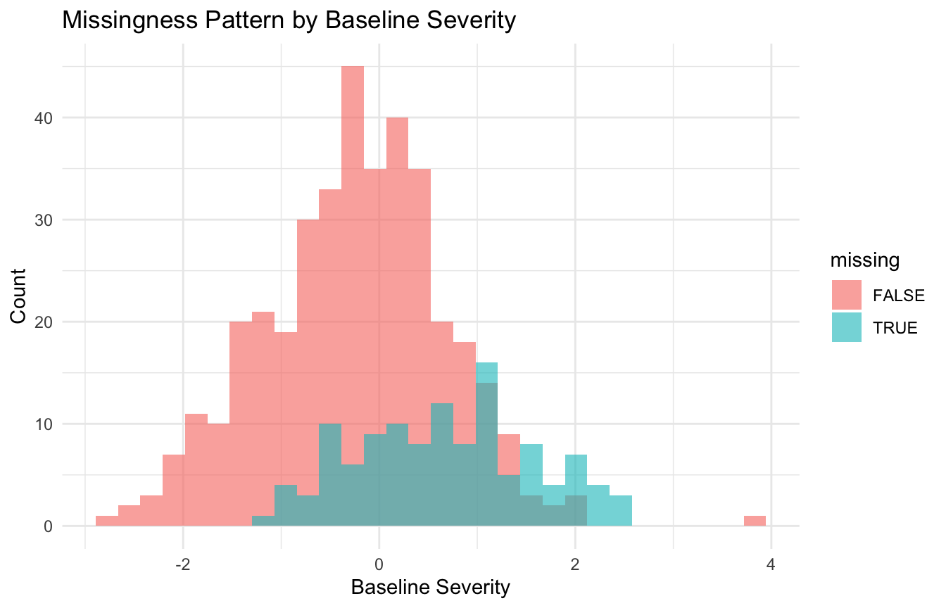
Here, missingness is related to an observed variable, baseline_severity.
That makes it MAR, not MCAR.
The important point is that the missingness is systematic, but potentially modelable. ## Simulating MNAR Shows Missingness Driven by the Unobserved Outcome
Now let us create an MNAR mechanism by making missingness more likely when the outcome itself is poor.
Little’s test can be useful, but it should be interpreted as one diagnostic among many, not as a final oracle. ## Logistic Missingness Models Are Often More Informative Than One Test Alone
Another practical strategy is to model the missingness indicator itself.
For example, define:
1 = outcome missing
0 = outcome observed
and regress that missingness indicator on observed variables.
Call:
glm(formula = missing ~ age + baseline_severity + treatment,
    family = binomial(), data = miss_model_df)

Coefficients:
                    Estimate Std. Error z value Pr(>|z|)
(Intercept)        -0.945059   0.583478  -1.620    0.105
age                -0.007575   0.009783  -0.774    0.439
baseline_severity   1.097176   0.138195   7.939 2.03e-15 ***
treatmentTreatment -0.051768   0.231286  -0.224    0.823
---
Signif. codes:  0 '***' 0.001 '**' 0.01 '*' 0.05 '.' 0.1 ' ' 1

(Dispersion parameter for binomial family taken to be 1)

    Null deviance: 546.43  on 499  degrees of freedom
Residual deviance: 463.77  on 496  degrees of freedom
AIC: 471.77

Number of Fisher Scoring iterations: 5
If observed variables strongly predict missingness, MCAR becomes less plausible.
This does not prove MAR, but it gives a more grounded sense of what the missingness process may depend on. ## MCAR, MAR, and MNAR Are Assumptions About the Data-Generating Process
One of the most important conceptual points is that these categories are not always directly testable from the observed data alone.
MCAR can sometimes be challenged empirically. MAR and MNAR are more difficult.
In practice:
MAR is often a working assumption,
MNAR is often a sensitivity concern,
and the real mechanism is rarely known with certainty.
This means missing-data analysis requires both:
diagnostics,
and subject-matter reasoning.
A purely mechanical classification approach is usually too simplistic. ## Missingness Mechanisms Matter for Imputation Strategy
Why does all this matter so much in AI/ML workflows?
Because the mechanism affects what imputation or modeling strategy is defensible.
For example:
Under MCAR
Simple methods may sometimes be less harmful, though efficiency is still lost.
Under MAR
Methods like multiple imputation or model-based imputation can be appropriate if the observed predictors of missingness are included (Rubin 1987; Buuren 2018).
Under MNAR
Standard imputation under MAR may still be biased, and sensitivity analysis becomes much more important.
This is why mechanism and imputation cannot be separated. The imputation model is only as good as the missingness assumptions behind it. ## Complete-Case Analysis Is Often Easy, but Often Too Optimistic
A common default is complete-case analysis: analyze only rows without missing data.
This can be acceptable under true MCAR, but it can be problematic under MAR or MNAR.
Problems include:
biased estimates,
distorted subgroup representation,
reduced power,
and unfair exclusion of under-measured populations.
This is especially important in predictive healthcare analytics, where complete-case filtering can quietly remove exactly the patients with the most complex or clinically important trajectories.
So complete-case analysis should be viewed as a modeling choice with assumptions, not as a neutral default. ## Missingness Indicators Can Sometimes Add Predictive Value
In predictive modeling, it is sometimes useful to include an indicator that a value was missing.
# A tibble: 2 × 2
  outcome_missing     n
  <lgl>           <int>
1 FALSE             382
2 TRUE              118
A missingness indicator does not solve the missing-data problem by itself. But it can sometimes help the model learn that the fact of missingness carries signal.
This is especially relevant in ML pipelines where missingness may reflect workflow, severity, or system context.
That said, missingness indicators should complement, not replace, careful thinking about mechanism. ## Python and R Both Support Practical Missingness Diagnostics
The missing-data workflow is not language-specific.
In R, analysts often use:
naniar
VIM
mice
BaylorEdPsych
Amelia
In Python, comparable workflows often involve:
pandas for missingness summaries
missingno for visualization
statsmodels or sklearn for missingness modeling
custom simulation and imputation pipelines
The core statistical questions remain the same in both ecosystems:
what is missing?
why is it missing?
and what assumptions are being made when we fill or ignore it? ## A Practical Checklist for Applied Work
Before choosing a missing-data strategy, ask:
Which variables are missing, and how often?
Do observed variables predict missingness?
Is MCAR plausible, or clearly implausible?
Is MAR a defensible working assumption?
Could the missingness plausibly depend on the unobserved value itself?
What would complete-case analysis exclude?
Does the imputation model include variables related to both missingness and the outcome?
Do I need sensitivity analysis for possible MNAR behavior?
These questions usually improve missing-data work more than rushing straight to imputation.
NoteWhere This Shows Up in AI/ML
In DoDTR-based mortality models, prehospital vital signs and mechanism-of-injury fields are frequently absent not at random but because they were never recorded in the chaos of point-of-injury care — a textbook MNAR scenario. A model trained without accounting for this mechanism can learn that missing prehospital data predicts survival, inverting the true clinical signal. Epic’s deterioration index faces the same problem: lab values are missing because the clinician didn’t order them, often because the patient appeared stable, creating a systematic association between missingness and perceived low risk. When the missingness mechanism is misclassified as MCAR and treated as ignorable, every downstream imputation, weighting, and inference step is built on a false foundation.
Closing: Missing Data Is About Mechanism, Not Just Percentage
Missing data analysis starts to improve when we stop asking only how much data are missing and start asking why the values are missing.
MCAR, MAR, and MNAR are not just vocabulary terms. They are different assumptions about the missingness process, and those assumptions shape what kind of inference or prediction is defensible.
In real-world AI and healthcare analytics, this matters because missingness is often informative. It reflects people, processes, systems, and outcomes — not just blank cells in a table.
Missing-data mechanisms matter because absent values still carry information, and the process that creates missingness can bias a model just as much as the values themselves.
This post is part of the Missing Data Toolkit — a companion reference with missingness mechanism diagnostics, Little’s MCAR test templates, and workflow scaffolds for handling MCAR, MAR, and MNAR in clinical data.
Little, Roderick J. A. 1988. “A Test of Missing Completely at Random for Multivariate Data with Missing Values.”Journal of the American Statistical Association 83 (404): 1198–202. https://doi.org/10.1080/01621459.1988.10478722.