Filling the Gaps: Imputation Strategies for Bulletproof ML Models
Advanced Statistics
Imputation
A practical guide to single imputation, KNN imputation, and multiple imputation, with evaluation strategies for machine learning and healthcare data.
Published
October 15, 2025
Modified
June 9, 2026
Executive Summary
Once missing data exist, analysts face a practical decision:
what should be done with the missing values before modeling?
This is where imputation techniques come in.
Imputation is the process of filling in missing values with plausible replacements so that analysis or prediction can proceed (Rubin 1987; Buuren 2018). But not all imputation methods are equally defensible, and not all are designed for the same goal.
Some methods are simple and fast:
mean imputation,
median imputation,
or mode imputation.
Others are more model-based:
K-nearest neighbors imputation,
regression-style imputation,
or multiple imputation by chained equations.
The key point is that imputation is not only a data-cleaning step. It is a modeling choice.
and how to think about continuous and categorical variables differently.
Imputation matters because filling in missing data is never neutral — every imputation method encodes assumptions about what the missing values probably were. ## Imputation Begins After the Missingness Question, Not Before It
A common mistake is to jump immediately from:
“there are missing values”
to:
“which imputation function should I run?”
That skips the most important first step.
Before imputing, the analyst should ask:
why are values missing?
which variables are affected?
are the missing values likely MCAR, MAR, or possibly MNAR?
is the goal inference, prediction, or both?
Imputation does not stand alone. It depends on the missingness mechanism and the modeling objective.
That is why imputation belongs after the missing-data diagnosis, not before it. ## Single Imputation Is Simple, but Usually Incomplete
Single imputation replaces each missing value with one filled-in value (Little and Rubin 2019).
Examples include:
mean imputation,
median imputation,
mode imputation,
or a single KNN-based estimate.
These approaches are attractive because they are easy to implement and fast to explain.
they usually do not reflect uncertainty about the missing value.
Once a single value is inserted, the analysis proceeds as if that value were known exactly.
That can make inference look more precise than it should.
This is one reason simple imputation is often more appropriate for prediction pipelines than for formal inferential settings. ## Mean Imputation Is Easy, but It Distorts Variation
The simplest possible imputation method for a continuous variable is mean imputation.
For every missing value, replace it with the observed mean of that variable.
That is convenient, but it comes at a cost.
Mean imputation tends to:
reduce variability,
attenuate relationships,
distort distributions,
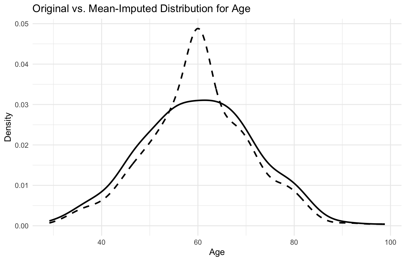
and create artificial spikes at the mean.
This makes it easy to implement but statistically blunt.
Still, it can serve as a useful baseline for comparison. ## A Small Example Makes the Comparison Concrete
To make the methods tangible, we will simulate a small healthcare-style dataset with both continuous and categorical variables.
Then we will hide some values artificially so we can compare imputation strategies against the known truth.
Now we will artificially mask some values so that we can evaluate how well the imputation methods recover them. ## Artificial Masking Makes Imputation Evaluation Possible
In real data, the true missing values are unknown. That makes direct evaluation difficult.
A common benchmarking strategy is:
start with a complete dataset,
hide a subset of values artificially,
impute them,
compare imputed values to the true original values.
This is especially useful for teaching and method comparison.
This is fast and often sufficient for very rough baselines, but it should rarely be treated as the final answer without justification. ## Simple Imputation Is Easy to Visualize — and Easy to Critique
One useful way to see the effect of simple imputation is to compare distributions before and after imputation.
This type of plot often reveals how simple imputation pulls the distribution toward the center and reduces natural variation. ## KNN Imputation Uses Similar Observations to Fill Gaps
K-nearest neighbors (KNN) imputation uses the values of similar observations to estimate missing entries.
The idea is:
find observations that are close based on other available variables
use those neighbors to fill in the missing value
This can be more flexible than simple mean imputation because it uses multivariable structure.
KNN imputation often works well when:
similar cases really do exist,
the feature space is well scaled,
and the data are not too sparse.
It can be especially useful in prediction pipelines, though it can become computationally heavy in larger datasets.
The exact choice of k matters and should usually be tuned or at least justified. ## KNN Imputation Requires Care with Scaling and Variable Types
Because KNN depends on similarity, it is sensitive to how distance is computed.
That means analysts need to think carefully about:
scaling continuous variables,
encoding categorical variables,
and whether the nearest neighbors are meaningful in the feature space.
If one variable dominates the scale, it can dominate the neighbor search too.
This is one reason KNN imputation can be helpful, but also somewhat fragile if preprocessing is poor.
In high-dimensional settings, the curse of dimensionality can also weaken neighborhood quality. ## Multiple Imputation Tries to Reflect Uncertainty, Not Just Fill Values
Multiple imputation takes a different approach.
Instead of creating one filled-in dataset, it creates several.
Each imputed dataset contains slightly different plausible replacements for the missing values, reflecting uncertainty about what those values might have been.
The general logic is:
generate multiple imputed datasets
analyze each one separately
pool the results across them
This is especially valuable for inference because it acknowledges that the imputed values are not known with certainty.
That is one reason multiple imputation is often considered a gold-standard working approach under MAR. ## MICE Is One of the Most Common Multiple Imputation Workflows
A widely used multiple imputation framework is MICE:
Multiple Imputation by Chained Equations
The idea is to iteratively model each incomplete variable conditional on the others.
This works well because different variable types can be handled with different conditional models.
For example:
predictive mean matching for continuous variables
logistic models for binary variables
multinomial models for unordered categorical variables
In R, the mice package is a standard tool for this workflow.
This produces multiple completed datasets rather than one single “final” imputed version. ## Multiple Imputation Is Stronger for Inference Than Single Imputation
One of the biggest reasons to prefer multiple imputation over simple single imputation in many inferential settings is that it better reflects uncertainty.
Single imputation acts as though the filled values are known. Multiple imputation treats them as uncertain.
This matters because confidence intervals and standard errors should reflect:
uncertainty from the observed data,
and uncertainty from the missing-value replacement process.
That is why multiple imputation is often much more defensible for regression, hypothesis testing, and effect estimation than simple mean imputation alone. ## Continuous and Categorical Variables Need Different Imputation Logic
Not all variables should be imputed the same way.
Continuous variables
Common choices include:
mean imputation
median imputation
predictive mean matching
KNN
regression-based models
Categorical variables
Common choices include:
mode imputation
logistic or multinomial imputation models
tree-based or KNN approaches
This distinction matters because the imputed values should respect the variable type.
For example:
a categorical variable should not be imputed with impossible hybrid values
a skewed continuous variable may be better handled with predictive mean matching than with a Gaussian assumption
Good imputation respects the measurement scale. ## RMSE on Masked Values Is a Useful Benchmark for Continuous Variables
When comparing imputation methods on masked continuous values, one simple evaluation metric is RMSE.
[ RMSE = ]
Because we deliberately hid known values, we can compare imputed estimates against truth.
For mean/median-style imputation, that looks like this.
# A tibble: 3 × 2
  variable rmse_simple
  <chr>          <dbl>
1 age           13.3
2 bmi            5.94
3 lactate        0.819
This provides a practical benchmarking framework even when the imputation method is simple. ## Classification Error Can Benchmark Categorical Imputation
For categorical variables, RMSE is not appropriate. Instead, we can compare the imputed class to the true masked class.
# A tibble: 1 × 2
  variable simple_imputation_accuracy
  <chr>                         <dbl>
1 sex                            0.45
This helps reinforce an important point: evaluation should match the variable type and the analytic goal. ## Imputation Quality Is Not the Same as Downstream Model Quality
A subtle but important point is that the “best” imputation method for recovering missing values is not always the same as the “best” method for downstream prediction.
Sometimes a method with lower masked-value RMSE may not yield the best predictive model. Conversely, a method that preserves model performance well may still distort some variable-level properties.
That is why imputation can be evaluated from at least two perspectives:
reconstruction quality
downstream model utility
Good applied work often considers both. ## Imputation Should Usually Be Embedded in the Modeling Pipeline
A major best practice in machine learning is to avoid imputing the full dataset before splitting into training and testing.
Why?
Because that can leak information.
Instead, the imputation process should usually be fit on the training data and then applied to validation or test data.
This is especially important for methods such as:
mean/median imputation,
KNN imputation,
and model-based imputation.
Imputation is part of preprocessing, and preprocessing belongs inside the resampling pipeline when performance is being evaluated honestly. ## Public Datasets Are Useful for Benchmarking, but Simulation Teaches Mechanism More Clearly
For blog posts and teaching, public datasets are often useful because they are familiar and reproducible.
But simulation has a major advantage:
the true masked values are known
and the missingness mechanism can be controlled
That makes simulation especially powerful for understanding:
what a method is really doing,
how imputation behaves under MCAR or MAR-like settings,
and how distributional assumptions affect the result.
For an educational post, a simulated clinical or RWE-style example is often clearer than a public dataset with unknown truth. ## Imputation Does Not Solve MNAR by Itself
One of the most important cautions is that imputation methods do not magically solve missingness caused by MNAR processes.
If missingness depends on the unseen value itself, then standard methods based on observed-data assumptions may still be biased.
That means:
mean imputation will not rescue the problem
KNN will not rescue the problem
and even multiple imputation under MAR may still miss the true mechanism
This is why imputation must always be interpreted in the context of the missingness mechanism.
The method is never more valid than the assumptions that justify it. ## A Practical Checklist for Applied Work
Before choosing an imputation strategy, ask:
What is the likely missingness mechanism?
Is the goal prediction, inference, or both?
Are variables continuous, categorical, or mixed?
Is a simple baseline enough, or is uncertainty modeling needed?
Would KNN meaningfully exploit local structure?
Is multiple imputation more appropriate under the working assumptions?
How will imputation quality be evaluated?
Is imputation being fit inside the validation pipeline to avoid leakage?
These questions usually matter more than choosing the fanciest method by default.
NoteWhere This Shows Up in AI/ML
Most clinical risk scores deployed in EHR systems — including trauma triage tools built on DoDTR data — use mean or median imputation because it is simple to implement and survives the engineering pipeline to production. The cost is understated uncertainty: a single imputed value carries no variance, so the model acts as if it knows something it does not, and calibration curves drift in patients where missingness is heaviest. MICE-based multiple imputation is standard in research submissions but is almost never reproduced in the deployed scoring function, creating a silent discrepancy between the validated model and the live one. When imputation strategy changes between training and deployment, apparent model performance is not real performance.
Closing: Imputation Is a Modeling Choice, Not a Neutral Repair Step
Imputation remains one of the most important practical tools in missing-data workflows because real datasets are rarely complete and many models cannot operate sensibly on missing inputs.
But imputation is not just gap-filling.
It changes the data representation and encodes assumptions about what unobserved values might have been.
Mean and median imputation are simple but blunt. KNN can use local structure but depends on meaningful similarity. Multiple imputation offers a stronger inferential framework by reflecting uncertainty across multiple plausible completed datasets.
Imputation matters because missing values are not just absent numbers, and how we replace them can shape everything the model learns afterward.
This post is part of the Missing Data Toolkit — a companion reference with single and multiple imputation templates, MICE workflow scaffolds, KNN imputation code, and pipeline embedding guidance.