RCTs: The Cornerstone of Evidence – Why AI Needs Controlled Chaos

Design of Experiments

A practical introduction to randomized controlled trials, randomization, allocation, crossover designs, and why design remains central to causal evidence in AI and clinical research.

Published

January 1, 2026

Modified

June 9, 2026

Executive Summary

Randomized controlled trials, or RCTs, remain the benchmark for causal evidence in clinical and applied research (Sibbald and Roland 1998; Friedman et al. 2015).

That is not because they are perfect. It is because, when designed well, they do something observational studies struggle to do:

make treatment assignment independent of the patient characteristics that would otherwise bias the comparison.

This is the central power of randomization (Friedman et al. 2015).

In an RCT, the treatment groups should differ mainly because of chance, not because one group was sicker, older, more adherent, or more likely to receive a clinician’s preferred intervention.

That design feature makes RCTs the cleanest setting for estimating causal effects.

This matters in both biostatistics and AI/ML.

In biostatistics, RCTs remain the gold standard for efficacy questions. In AI/ML, they provide clean intervention data that can anchor baseline causal models, validate treatment-response hypotheses, and contrast sharply with messier real-world evidence.

This post introduces:

why randomization matters,
how parallel-group and crossover trials differ,
what allocation ratios do,
and how simulation can show the difference between randomized and non-randomized comparisons.

RCTs matter because good causal evidence does not begin with complicated modeling, but with a design that makes the treatment comparison fair from the start.

1. RCTs Begin with a Simple Problem: Treatment Groups Are Usually Not Comparable

In routine practice, treatment is rarely assigned randomly.

Patients receive one treatment rather than another because of:

disease severity,
clinician judgment,
access,
preference,
contraindications,
timing,
or site-level practice patterns.

That means treatment groups often differ before the treatment effect is ever observed.

If we compare them naively, we risk attributing those baseline differences to the treatment itself.

This is the core problem randomization is designed to solve.

2. Randomization Minimizes Bias by Breaking Systematic Assignment

The defining feature of an RCT is that treatment assignment is randomized.

That means, at the point of assignment, no patient characteristic should systematically determine who receives which intervention.

In expectation, randomization balances both:

measured variables,
and unmeasured variables.

This is what makes RCTs so powerful for causal inference.

It does not guarantee that groups are exactly identical in every realized sample. Chance imbalance can still occur.

But it removes systematic assignment bias, which is the more dangerous problem.

That is why randomization is often described as the cleanest design solution to confounding.

3. Randomization Does Not Eliminate Noise — It Eliminates Predictable Bias

A useful way to understand RCTs is this:

randomization does not make the data noiseless,
it makes the treatment comparison unbiased in expectation.

In other words:

outcomes can still vary,
small trials can still be imbalanced by chance,
and estimates can still be imprecise,

but the treatment difference is not systematically driven by the same kinds of assignment processes that distort observational studies.

That is a major distinction.

RCTs do not remove uncertainty. They remove one of the most damaging sources of structured bias.

4. A Parallel-Group Trial Is the Standard RCT Design

The most common RCT design is the parallel-group trial.

In a parallel-group RCT:

one group receives treatment A,
another group receives treatment B or control,
and each participant remains in that assigned arm for follow-up.

This design is common because it is:

conceptually simple,
broadly applicable,
and relatively easy to analyze.

It works especially well when:

the intervention has a lasting effect,
carryover would be problematic,
or the disease process is not stable enough for within-person crossover comparison.

For many readers, this is the default mental model of an RCT.

5. Crossover Trials Ask a Different Kind of Question

A crossover trial assigns participants to receive multiple treatments in sequence.

For example:

one group may receive A then B,
another may receive B then A.

This allows each participant to serve as their own control.

That can be powerful because it reduces between-person variability.

But crossover designs only work well under specific conditions, such as:

a stable condition,
reversible treatment effects,
and adequate washout periods.

If carryover effects are likely, crossover designs can become misleading.

So crossover trials are not a superior version of RCTs in general. They are a specialized design for the right setting.

6. Allocation Ratios Affect Efficiency and Practicality

Another important design choice is the allocation ratio.

The most familiar ratio is:

1:1 treatment to control

This is often statistically efficient when group costs are similar.

But other ratios may be used, such as:

2:1
3:1
or more complex multi-arm allocations

Why would this happen?

Possible reasons include:

ethical preference for giving more participants access to an experimental treatment,
logistical constraints,
safety data collection goals,
or unequal treatment costs.

The key tradeoff is that unequal allocation may reduce statistical efficiency for a fixed total sample size, though it may improve feasibility or acceptability.

7. A Simple Allocation Example Makes the Arithmetic Concrete

Let us create a simple allocation example for a two-arm trial.

n_total <- 300

alloc_1_1 <- tibble::tibble(
  arm = c("Control", "Treatment"),
  proportion = c(0.5, 0.5),
  n_assigned = c(0.5, 0.5) * n_total
)

alloc_2_1 <- tibble::tibble(
  arm = c("Control", "Treatment"),
  proportion = c(1/3, 2/3),
  n_assigned = c(1/3, 2/3) * n_total
)

alloc_1_1

# A tibble: 2 × 3
  arm       proportion n_assigned
  <chr>          <dbl>      <dbl>
1 Control          0.5        150
2 Treatment        0.5        150

alloc_2_1

# A tibble: 2 × 3
  arm       proportion n_assigned
  <chr>          <dbl>      <dbl>
1 Control        0.333        100
2 Treatment      0.667        200

This makes the allocation-ratio idea concrete before it becomes embedded in simulation or power calculations.

8. Simulating an RCT Helps Show Why Randomization Works

One of the best ways to understand RCTs is to simulate them.

We will create a scenario in which baseline severity affects outcome, but treatment assignment is randomized.

This lets us see how a randomized design protects the treatment comparison from severity-based confounding.

library(dplyr)
library(tibble)
library(ggplot2)

n <- 500

rct_df <- tibble::tibble(
  id = 1:n,
  age = rnorm(n, mean = 60, sd = 12),
  baseline_severity = rnorm(n, mean = 0, sd = 1),
  treatment = rbinom(n, size = 1, prob = 0.5)
) |>
  dplyr::mutate(
    outcome = 50 + 3 * treatment - 4 * baseline_severity - 0.1 * age + rnorm(n, 0, 5)
  )

In this simulated RCT, treatment has a real beneficial effect of 3 units on the outcome.

Because assignment is random, baseline severity should be roughly balanced across arms.

9. Randomization Usually Produces Balance, Even If Not Perfectly

Let us inspect the treatment groups.

rct_df |>
  dplyr::group_by(treatment) |>
  dplyr::summarise(
    n = dplyr::n(),
    mean_age = mean(age),
    mean_baseline_severity = mean(baseline_severity),
    .groups = "drop"
  )

# A tibble: 2 × 4
  treatment     n mean_age mean_baseline_severity
      <int> <int>    <dbl>                  <dbl>
1         0   259     60.2                 0.0361
2         1   241     59.4                -0.0899

The groups may not be exactly equal, but they should be reasonably similar.

That is a major design achievement.

In a nonrandomized setting, these kinds of differences could be much larger and systematically aligned with prognosis.

10. The Treatment Effect in an RCT Can Be Estimated Transparently

Because treatment assignment is randomized, the treatment effect can often be estimated with a relatively simple comparison.

rct_df |>
  dplyr::group_by(treatment) |>
  dplyr::summarise(
    mean_outcome = mean(outcome),
    .groups = "drop"
  ) |>
  tidyr::pivot_wider(
    names_from = treatment,
    values_from = mean_outcome
  ) |>
  dplyr::mutate(
    estimated_treatment_effect = `1` - `0`
  )

# A tibble: 1 × 3
    `0`   `1` estimated_treatment_effect
  <dbl> <dbl>                      <dbl>
1  44.0  46.9                       2.89

This is one of the key strengths of RCTs.

The design does so much causal work that the analysis can often remain comparatively straightforward.

11. Now Compare That with a Non-Randomized Assignment Mechanism

To show why randomization matters, let us simulate a second dataset in which sicker patients are more likely to receive treatment.

obs_df <- tibble::tibble(
  id = 1:n,
  age = rnorm(n, mean = 60, sd = 12),
  baseline_severity = rnorm(n, mean = 0, sd = 1)
) |>
  dplyr::mutate(
    treat_prob = plogis(-0.2 + 1.2 * baseline_severity),
    treatment = rbinom(n, size = 1, prob = treat_prob),
    outcome = 50 + 3 * treatment - 4 * baseline_severity - 0.1 * age + rnorm(n, 0, 5)
  )

The true treatment effect is still 3. But now treatment assignment depends on severity.

That means the crude comparison will be biased.

12. The Non-Randomized Comparison Mixes Effect and Confounding

Let us compare the groups.

obs_df |>
  dplyr::group_by(treatment) |>
  dplyr::summarise(
    n = dplyr::n(),
    mean_age = mean(age),
    mean_baseline_severity = mean(baseline_severity),
    .groups = "drop"
  )

# A tibble: 2 × 4
  treatment     n mean_age mean_baseline_severity
      <int> <int>    <dbl>                  <dbl>
1         0   249     59.8                 -0.320
2         1   251     60.2                  0.551

Now estimate the naïve treatment effect.

obs_df |>
  dplyr::group_by(treatment) |>
  dplyr::summarise(
    mean_outcome = mean(outcome),
    .groups = "drop"
  ) |>
  tidyr::pivot_wider(
    names_from = treatment,
    values_from = mean_outcome
  ) |>
  dplyr::mutate(
    naive_treatment_effect = `1` - `0`
  )

# A tibble: 1 × 3
    `0`   `1` naive_treatment_effect
  <dbl> <dbl>                  <dbl>
1  46.2  45.0                  -1.24

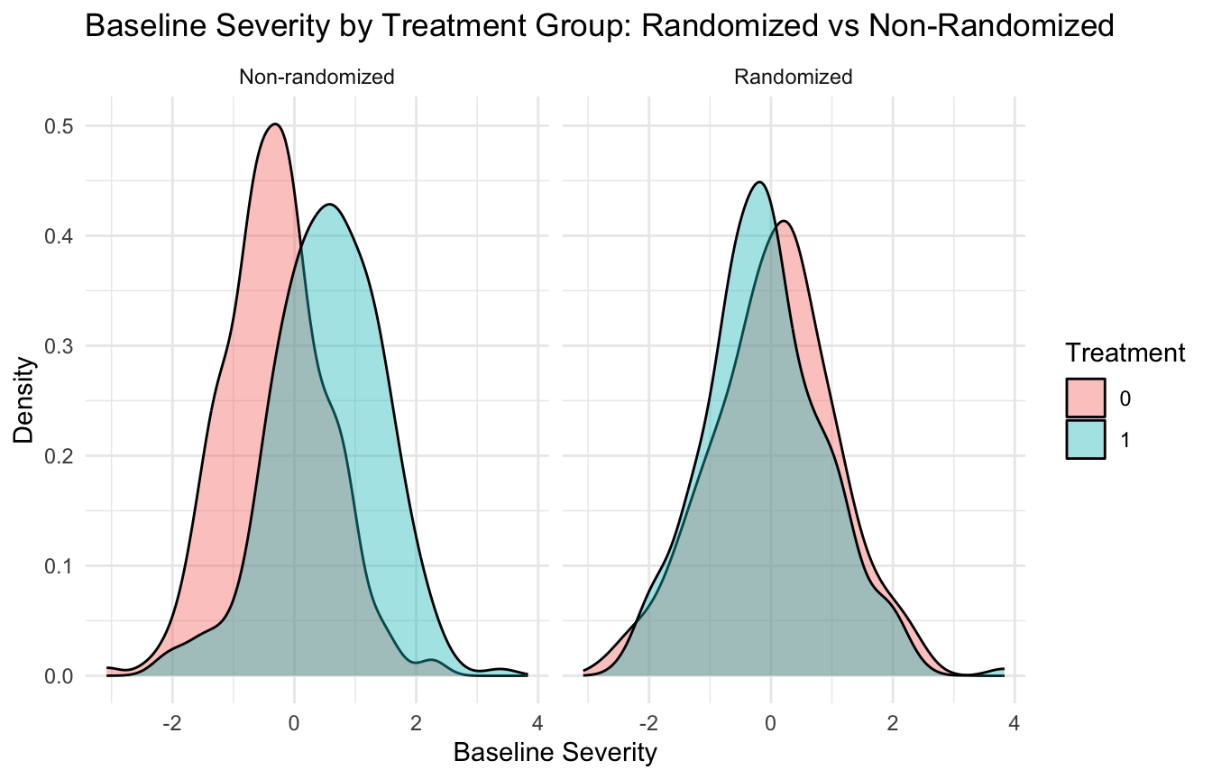
Even though the true effect remains +3, the observational estimate may be much smaller or even misleading because sicker patients were more likely to receive treatment.

This is the main contrast the blog title is pointing toward:

controlled chaos beats uncontrolled selection.

13. Visualization Helps Make the Contrast Immediate

A simple plot can show the difference in baseline severity across designs.

plot_rct <- rct_df |>
  dplyr::mutate(design = "Randomized")

plot_obs <- obs_df |>
  dplyr::mutate(design = "Non-randomized")

plot_df <- dplyr::bind_rows(plot_rct, plot_obs)

ggplot2::ggplot(plot_df, ggplot2::aes(x = baseline_severity, fill = factor(treatment))) +
  ggplot2::geom_density(alpha = 0.4) +
  ggplot2::facet_wrap(~ design) +
  ggplot2::labs(
    title = "Baseline Severity by Treatment Group: Randomized vs Non-Randomized",
    x = "Baseline Severity",
    y = "Density",
    fill = "Treatment"
  ) +
  ggplot2::theme_minimal()

This kind of figure often teaches more quickly than paragraphs of description.

14. RCTs Are the Gold Standard for Causal Inference, but Not for Every Question (Sibbald and Roland 1998)

RCTs are powerful because they solve a major causal problem at the design stage.

But that does not mean they are automatically ideal for every question.

RCTs can still be limited by:

cost,
narrow eligibility criteria,
short follow-up,
ethical constraints,
nonadherence,
and limited external validity.

So the real lesson is not:

“RCTs are always enough.”

It is:

“RCTs provide the cleanest causal benchmark.”

That is why they remain the reference design even when later work must move into pragmatic or real-world settings.

15. RCTs Matter in AI/ML Because They Provide Clean Intervention Data

In AI/ML, RCTs matter because they produce data where treatment assignment is not tangled up with the same observational biases that plague real-world datasets.

This makes RCT data valuable for:

benchmarking treatment-response models,
validating causal assumptions,
estimating cleaner baseline effects,
and contrasting trial evidence with real-world deployment data.

For example, a model predicting drug efficacy may benefit from trial-derived labels precisely because the assignment mechanism is known and controlled.

That does not mean trial data alone are always enough for deployment. But they provide a strong anchor.

16. Hybrid Evidence Strategies Often Compare RCTs with RWE

A very important modern theme is that RCTs and real-world evidence are not enemies.

They answer different parts of the evidence problem.

RCTs are strong for:

internal validity,
efficacy,
and causal clarity.

RWE is often stronger for:

broader populations,
routine-care settings,
implementation variation,
and long-term use patterns.

This is why hybrid evidence approaches matter so much in AI and biostatistics. RCTs often define the causal core. RWE tests transportability, heterogeneity, and practical deployment.

17. Intent-to-Treat Thinking Starts in RCTs

One reason RCTs are so foundational methodologically is that they introduce ideas like intent-to-treat (Friedman et al. 2015; Moher et al. 2010).

Intent-to-treat analysis compares participants according to their randomized assignment, regardless of later adherence.

This preserves the causal benefit of randomization.

That is an important lesson because post-randomization behavior can reintroduce bias if handled carelessly.

Even when the main blog post does not go deep into adherence or attrition, it helps to mention that trial design and trial analysis are linked.

The causal strength of an RCT depends partly on preserving the logic of the assignment process in the analysis.

18. Small Trials Can Still Show Chance Imbalance

A useful caution is that randomization does not guarantee perfect balance in a single realized sample, especially in smaller trials.

This is why analysts still:

inspect baseline summaries,
consider stratification or blocking,
and interpret small-sample imbalances carefully.

The point is not that imbalance means the RCT failed. It means randomization eliminates systematic bias, not all observed difference.

That distinction matters for both teaching and interpretation.

19. A Practical Checklist for Applied Work

Before designing or interpreting an RCT, ask:

What exactly is being randomized?
Is the design parallel-group or crossover?
Is the allocation ratio appropriate?
Is time zero clearly defined?
Are important baseline covariates likely to be balanced by design, or should stratified randomization be used?
Is the estimand clear?
Will the analysis preserve the benefits of randomization?

These questions usually matter more than superficial trial labels.

Where This Shows Up in AI/ML

The stepped-wedge RCT is increasingly the design of choice for evaluating clinical AI deployment — a decision support tool rolls out across units sequentially, with each unit serving as its own control before exposure. This is how MAVEN-integrated triage decision support tools should be evaluated, not with single-site pre-post comparisons that confound the AI effect with temporal trends. Without randomization of rollout order, any observed improvement is as likely attributable to staff attention, concurrent training, or seasonal case mix as to the tool itself. Skipping this design for convenience produces AI “effectiveness” claims that cannot survive scrutiny when the system is proposed for wider fielding.

Closing: RCTs Earn Their Status by Making the Comparison Fair

Randomized controlled trials remain the cornerstone of evidence because they address a central causal problem directly:

they make treatment assignment fair in expectation.

That does not make them simple, cheap, or universally sufficient. But it does make them uniquely powerful.

Parallel-group and crossover designs answer different questions. Allocation ratios shape efficiency and feasibility. Simulation makes the main lesson visible:

when treatment is randomized, the comparison is cleaner
when it is not, the estimate can be distorted before the model even begins

RCTs matter because the most convincing evidence often comes not from more complicated analysis, but from a design that prevents bias from entering the treatment comparison in the first place.

📚 Go Deeper: Real-World Evidence Toolkit

This post is part of the Real-World Evidence Toolkit — a companion reference with RCT reporting checklists, intent-to-treat analysis templates, and hybrid RCT/RWE comparison scaffolds.

→ Open the Real-World Evidence Toolkit

Series Callout

Note

This post concludes the series on Design of Experiments for Biostats and AI/ML:

Randomized controlled trials
Observational study designs
Cross-sectional study design
Longitudinal study design
Sample size and power analysis
Stratification and randomization techniques
Blinding and placebo controls
Adaptive study designs
Pragmatic trials
Quasi-experimental designs

Series: Design of Experiments

Observational Power: Turning Real-World Data into AI Goldmines →

References

Friedman, Lawrence M., Curt D. Furberg, David L. DeMets, David M. Reboussin, and Christopher B. Granger. 2015. Fundamentals of Clinical Trials. 5th ed. Springer.

Moher, David, Sally Hopewell, Kenneth F. Schulz, et al. 2010. “CONSORT 2010 Explanation and Elaboration: Updated Guidelines for Reporting Parallel Group Randomised Trials.” BMJ 340: c869. https://doi.org/10.1136/bmj.c869.

Sibbald, Bonnie, and Martin Roland. 1998. “Understanding Controlled Trials: Why Are Randomised Controlled Trials Important?” BMJ 316 (7126): 201. https://doi.org/10.1136/bmj.316.7126.201.