Quasi Magic: Causal Insights Without RCTs for AI

Design of Experiments

A practical introduction to interrupted time series, difference-in-differences, regression discontinuity, and natural experiments for policy AI and real-world evidence.

Published

May 15, 2026

Modified

June 9, 2026

Executive Summary

Not every important intervention can be evaluated with a randomized trial.

Sometimes the intervention is:

a policy change,
a reimbursement reform,
a hospital workflow rollout,
a public-health mandate,
or a threshold-based eligibility rule.

In those settings, researchers often turn to quasi-experimental designs.

Quasi-experimental designs try to recover causal insight from observational data when randomization is unavailable, infeasible, or unethical. They do this by exploiting structure in time, policy timing, eligibility thresholds, or naturally occurring comparison groups.

This matters in both biostatistics and AI/ML.

In biostatistics and real-world evidence, quasi-experiments help estimate intervention effects from routine data. In AI/ML, they matter for policy evaluation, deployment monitoring, and causal assessment of interventions in real systems where randomized experimentation is limited.

This post introduces:

interrupted time series,
difference-in-differences,
regression discontinuity,
and the broader logic of natural experiments.

Quasi-experimental reasoning is foundational in applied causal inference because it tries to recover leverage from structure rather than from random assignment alone (Shadish et al. 2002; Bernal et al. 2017, 2019).

Quasi-experimental designs matter because sometimes the world changes in ways that are not randomized, but are still structured enough to support credible causal learning if analyzed carefully.

1. Quasi-Experiments Begin Where Randomization Is Missing

A quasi-experimental design is used when the analyst wants a causal interpretation but does not have randomized assignment.

That means the challenge is greater than in an RCT.

The key question becomes:

is there some structure in the data-generating process that can help separate intervention effects from ordinary background change?

Possible sources of that structure include:

a policy introduced at a known time,
a threshold that determines treatment eligibility,
one group exposed while another is not,
or a natural experiment that approximates assignment.

These designs are not magic. They still rely on assumptions.

But when the assumptions are plausible, they can bridge observational data toward causal reasoning (Shadish et al. 2002; Imbens and Rubin 2015).

2. Natural Experiments Are Valuable Because They Create Useful Variation

A natural experiment is not an experiment designed by the researcher. It is a real-world event or rule that creates variation in exposure in a way that may support causal inference.

Examples include:

a new hospital policy,
a state-level reimbursement change,
rollout of a digital alert system,
a cutoff for treatment eligibility,
or a sudden clinical guideline update.

These events are valuable because they may create contrasts that are more credible than ordinary uncontrolled observational comparisons.

That is why quasi-experimental designs often begin by identifying a real-world shock or discontinuity that changes exposure (Shadish et al. 2002; Angrist et al. 1996).

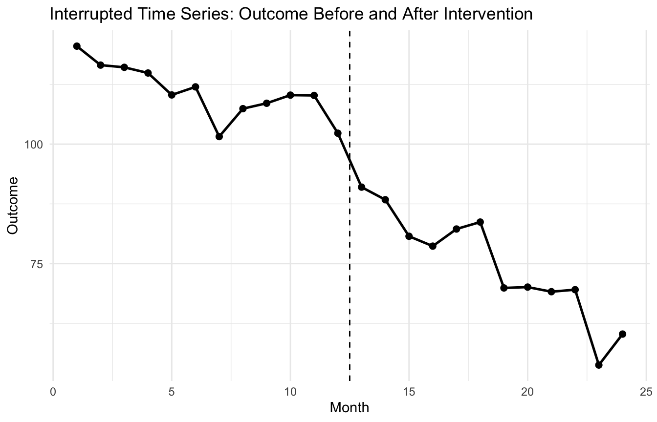
3. Interrupted Time Series Uses Time Itself as the Comparative Structure

An interrupted time series (ITS) design studies an outcome measured repeatedly over time before and after an intervention.

The idea is to ask:

what was the level and trend before the intervention?
what changed immediately after the intervention?
did the slope change afterward?

This is one of the most useful quasi-experimental approaches when a policy or system intervention affects an entire population at a known time.

ITS is especially strong when there are many time points both before and after the intervention.

That allows the pre-intervention trajectory to serve as a counterfactual trend.

4. A Policy Example Makes ITS Concrete

Suppose a healthcare system implements an AI-driven medication safety alert in month 13, and we want to study monthly adverse-event counts before and after the rollout.

We can simulate a time series with:

a baseline trend,
an intervention point,
and a post-intervention level and slope change.

library(dplyr)
library(tibble)
library(ggplot2)

n_months <- 24

its_df <- tibble::tibble(
  month = 1:n_months,
  post = if_else(month >= 13, 1, 0),
  time_after = if_else(month >= 13, month - 12, 0)
) |>
  dplyr::mutate(
    outcome = 120 +
      (-1.5 * month) +
      (-10 * post) +
      (-1.2 * time_after) +
      rnorm(n_months, 0, 4)
  )

its_df

# A tibble: 24 × 4
   month  post time_after outcome
   <int> <dbl>      <dbl>   <dbl>
 1     1     0          0    121.
 2     2     0          0    117.
 3     3     0          0    116.
 4     4     0          0    115.
 5     5     0          0    110.
 6     6     0          0    112.
 7     7     0          0    102.
 8     8     0          0    107.
 9     9     0          0    109.
10    10     0          0    110.
# ℹ 14 more rows

This simulates a series where the intervention reduces the outcome level and also changes the slope.

5. ITS Is Easy to Visualize and Often Best Introduced Graphically

A plot is often the clearest way to explain interrupted time series.

ggplot2::ggplot(its_df, ggplot2::aes(x = month, y = outcome)) +
  ggplot2::geom_line(linewidth = 0.9) +
  ggplot2::geom_point(size = 2) +
  ggplot2::geom_vline(xintercept = 12.5, linetype = 2) +
  ggplot2::labs(
    title = "Interrupted Time Series: Outcome Before and After Intervention",
    x = "Month",
    y = "Outcome"
  ) +
  ggplot2::theme_minimal()

This makes the intervention timing visible and helps separate:

the pre-existing trend,
the immediate level shift,
and the post-intervention trajectory.

That is one reason ITS is such a visually compelling quasi-experimental design.

6. Segmented Regression Is the Standard ITS Analysis

A common way to analyze ITS is with segmented regression.

The basic model often includes:

time
a post-intervention indicator
and time after intervention

This allows separate estimation of:

baseline slope
immediate level change
and post-intervention slope change

fit_its <- lm(
  outcome ~ month + post + time_after,
  data = its_df
)

summary(fit_its)$coefficients

              Estimate Std. Error   t value     Pr(>|t|)
(Intercept) 118.816535  2.5140264 47.261451 5.360472e-22
month        -1.220069  0.3415889 -3.571745 1.909597e-03
post        -10.623868  3.3526797 -3.168769 4.828068e-03
time_after   -1.667835  0.4830797 -3.452505 2.517005e-03

This is one of the most intuitive quasi-experimental models because each term has a direct interpretation tied to the intervention timeline.

7. ITS Is Stronger When It Controls for Pre-Existing Trends (Bernal et al. 2017)

One of the major strengths of interrupted time series is that it does not simply compare:

before average
versus after average

Instead, it controls for the fact that outcomes may already have been rising or falling before the intervention.

That is crucial.

A simple pre/post comparison can be badly misleading if the outcome was already trending downward before the intervention.

ITS improves on this by treating the pre-intervention trajectory itself as part of the causal comparison.

That is why trend control is central to the design.

8. Difference-in-Differences Adds a Comparison Group

A second major quasi-experimental approach is difference-in-differences (DiD).

DiD compares:

the change over time in an intervention group
versus the change over time in a comparison group

This helps control for shared background trends affecting both groups.

The key logic is:

if both groups would have followed parallel trends absent the intervention, then the extra change in the treated group can be attributed to the intervention (Bernal et al. 2019; Imbens and Rubin 2015).

That is the central identifying idea.

9. A Difference-in-Differences Example Makes the Logic Concrete

Suppose one hospital system adopts an AI triage intervention while another similar system does not.

We measure an outcome before and after the rollout in both groups.

did_df <- expand.grid(
  group = c("Control", "Treated"),
  period = c("Pre", "Post"),
  rep = 1:200
) |>
  tibble::as_tibble() |>
  dplyr::mutate(
    treated = if_else(group == "Treated", 1, 0),
    post = if_else(period == "Post", 1, 0),
    outcome = 50 +
      2 * treated +
      (-1) * post +
      (-4) * (treated * post) +
      rnorm(dplyr::n(), 0, 6)
  )

did_df |>
  dplyr::group_by(group, period) |>
  dplyr::summarise(
    mean_outcome = mean(outcome),
    .groups = "drop"
  )

# A tibble: 4 × 3
  group   period mean_outcome
  <fct>   <fct>         <dbl>
1 Control Pre            49.8
2 Control Post           49.9
3 Treated Pre            52.3
4 Treated Post           46.6

This setup creates a treated group that improves more after the intervention.

10. The DiD Estimator Is the Difference of Differences

The DiD estimate can be seen directly from group means:

[ ( - ) - ( - )]

We can compute it explicitly.

did_means <- did_df |>
  dplyr::group_by(group, period) |>
  dplyr::summarise(
    mean_outcome = mean(outcome),
    .groups = "drop"
  ) |>
  tidyr::pivot_wider(
    names_from = c(group, period),
    values_from = mean_outcome
  ) |>
  dplyr::mutate(
    did_estimate = (Treated_Post - Treated_Pre) - (Control_Post - Control_Pre)
  )

did_means

# A tibble: 1 × 5
  Control_Pre Control_Post Treated_Pre Treated_Post did_estimate
        <dbl>        <dbl>       <dbl>        <dbl>        <dbl>
1        49.8         49.9        52.3         46.6        -5.86

This is the core idea of DiD: compare changes, not just levels.

11. A Regression Formulation of DiD Makes It Easy to Extend

DiD is often implemented through a regression with an interaction term.

fit_did <- lm(
  outcome ~ treated + post + treated:post,
  data = did_df
)

summary(fit_did)$coefficients

               Estimate Std. Error    t value     Pr(>|t|)
(Intercept)  49.7520631  0.4283484 116.148601 0.000000e+00
treated       2.5298422  0.6057761   4.176200 3.291643e-05
post          0.1552877  0.6057761   0.256345 7.977507e-01
treated:post -5.8643165  0.8566967  -6.845265 1.524927e-11

The interaction term is the DiD estimator.

This formulation is useful because it extends naturally to:

covariate adjustment,
fixed effects,
multiple time periods,
and more complex policy settings.

12. The Parallel Trends Assumption Is the Core DiD Requirement

The most important assumption in DiD is parallel trends.

This means that, absent the intervention, the treated and control groups would have changed similarly over time.

That assumption cannot be proven directly for the unobserved counterfactual world. But it can sometimes be assessed indirectly by examining:

pre-intervention trends,
contextual similarity,
and plausibility of common shocks.

This is why DiD is powerful but not automatic. Its credibility depends heavily on whether the untreated comparison group is a good stand-in for the counterfactual trend.

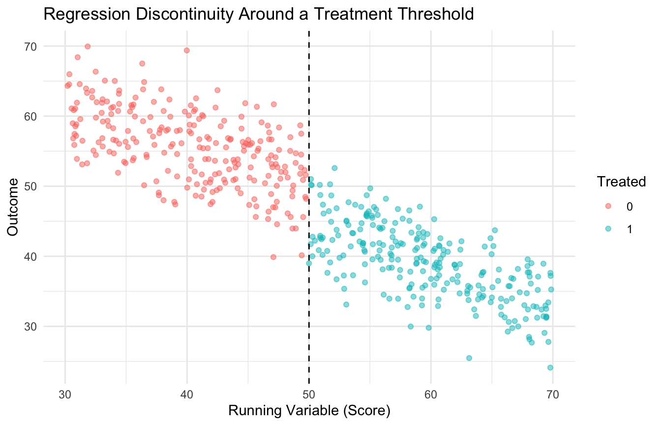
13. Regression Discontinuity Uses a Threshold as the Source of Causal Leverage

A third major quasi-experimental design is regression discontinuity (RD).

RD is used when treatment assignment changes sharply at a cutoff in a running variable.

Examples include:

age thresholds,
score cutoffs,
biomarker thresholds,
or eligibility rules for programs or intensified treatment.

The idea is that units just above and just below the cutoff are often similar except for treatment assignment.

That local contrast can support causal inference near the threshold.

14. A Simple RD Example Makes the Design Visible

Suppose a clinical support program is triggered when a risk score is at least 50.

We can simulate a setting where treatment jumps at that threshold and outcomes respond accordingly.

n_rd <- 500

rd_df <- tibble::tibble(
  score = runif(n_rd, min = 30, max = 70)
) |>
  dplyr::mutate(
    treated = if_else(score >= 50, 1, 0),
    outcome = 80 - 0.6 * score - 5 * treated + rnorm(n_rd, 0, 4)
  )

Now visualize the discontinuity.

ggplot2::ggplot(rd_df, ggplot2::aes(x = score, y = outcome, color = factor(treated))) +
  ggplot2::geom_point(alpha = 0.5) +
  ggplot2::geom_vline(xintercept = 50, linetype = 2) +
  ggplot2::labs(
    title = "Regression Discontinuity Around a Treatment Threshold",
    x = "Running Variable (Score)",
    y = "Outcome",
    color = "Treated"
  ) +
  ggplot2::theme_minimal()

This is the visual heart of RD: look for a jump at the cutoff.

15. A Simple RD Regression Can Capture the Local Jump

A basic linear RD model includes:

the running variable
the treatment indicator
and optionally an interaction with the running variable

fit_rd <- lm(
  outcome ~ score + treated + score:treated,
  data = rd_df
)

summary(fit_rd)$coefficients

                Estimate Std. Error      t value      Pr(>|t|)
(Intercept)   77.0548052 1.84793551  41.69777821 3.027535e-164
score         -0.5314402 0.04529451 -11.73299376  3.169379e-28
treated        0.3237753 3.31987383   0.09752638  9.223478e-01
score:treated -0.1102488 0.06457490  -1.70730115  8.839190e-02

The treatment term reflects the discontinuity at the cutoff under this specification.

In more formal work, analysts usually pay close attention to:

bandwidth selection,
local polynomial fit,
and robustness checks.

But for an introductory post, the key point is that the threshold creates the quasi-experimental leverage.

Trauma Registry Application: Quasi-Experiments for System-Level Interventions

Trauma systems are frequently changed by policy — but rarely by randomized experiment.

Classic trauma system interventions that are natural quasi-experimental settings:

Trauma center designation changes: when a hospital becomes a Level II center, interrupted time series can evaluate whether risk-adjusted mortality changed before and after designation.
Protocol adoptions: if a trauma network adopts a new massive transfusion protocol on a known date, ITS can estimate the effect on transfusion ratios and 30-day mortality.
Transfer policy changes: difference-in-differences can compare mortality trends at hospitals that changed transfer thresholds against those that did not.
Verification cycles: ACS trauma center verification has known renewal dates — a natural regression discontinuity around the verification score threshold.

Each of these requires the same careful design thinking as any quasi-experiment (Shadish et al. 2002; Bernal et al. 2017):

a credible counterfactual (what would have happened without the policy change?),
a plausible assumption about parallel trends or continuity around the threshold,
and documentation of potential co-interventions that coincide with the change.

Trauma registries — with their longitudinal, multi-center structure — are well suited to these designs when randomization is impossible.

16. Quasi-Experimental Designs Matter Because Policy and System Interventions Are Rarely Randomized

In many real-world healthcare and policy settings, interventions occur through:

regulation,
institutional rollout,
guideline changes,
reimbursement shifts,
and eligibility rules.

These are not randomized.

But they are also not always structureless.

Quasi-experimental designs matter because they exploit that structure to get closer to causal interpretation than a generic observational comparison would allow.

This is especially relevant in RWE and policy AI, where interventions are often system-level rather than patient-level randomized treatments.

17. AI/ML Benefits from Quasi-Experimental Thinking Too

In AI/ML, quasi-experimental designs are useful for questions such as:

did an alert reduce adverse events after rollout?
did a triage model change admission patterns?
did a policy algorithm alter utilization after implementation?
did a new risk score improve outcomes above and beyond background trends?

These are not only predictive questions. They are impact questions.

That means model performance metrics alone are often insufficient.

Quasi-experimental design helps evaluate whether an intervention changed the system, not just whether a model scores well retrospectively.

18. Real-World Policy Evaluation Often Depends on These Designs

A useful policy framing is that quasi-experimental methods are often the main analytic tools available when governments, hospitals, or health systems introduce interventions without randomized rollout.

Examples include:

a new prescribing regulation,
staffing policy change,
digital triage implementation,
reimbursement incentive,
or public-health campaign.

In those contexts, interrupted time series, DiD, and RD are often not optional extras. They are the main path from routine observational data to causal policy evaluation.

That is why they remain so important in applied evidence work.

19. Each Quasi-Experimental Design Has a Distinct Core Assumption

A useful summary is:

Interrupted time series

Needs a stable pre-intervention trend and no other major coincident shocks that explain the change.

Difference-in-differences

Needs parallel trends between treated and comparison groups absent the intervention.

Regression discontinuity

Needs a credible threshold rule and comparability of units near the cutoff.

These are not interchangeable assumptions. The design should match the structure of the intervention and the available data.

That is one reason quasi-experimental literacy matters so much.

20. A Practical Checklist for Applied Work

Before choosing a quasi-experimental design, ask:

Is there a clear intervention time, threshold, or comparison group?
Would interrupted time series control a trend better than a naïve pre/post comparison?
Is there a defensible comparison group for DiD?
Is the parallel trends assumption plausible?
Is there a meaningful cutoff for regression discontinuity?
Are there enough observations before and after the intervention?
Could other simultaneous changes explain the observed effect?

These questions usually matter more than the elegance of the final regression model.

Where This Shows Up in AI/ML

Difference-in-differences is the standard design for evaluating a clinical AI deployment when randomization was not done — comparing outcome trends before and after deployment at intervention sites against trends at control sites over the same period. MAVEN rollout evaluations, MHS GENESIS go-live analyses, and decision support implementation studies all require this structure to isolate AI effects from concurrent secular trends like staffing changes, protocol updates, or shifts in patient acuity. Without a control group providing the counterfactual trend, a pre-post comparison at a single site cannot distinguish “the model helped” from “outcomes were already improving.” The failure mode is deploying a clinical AI tool, observing better outcomes, and attributing improvement to the model when a DiD analysis with matched control MTFs would have shown the same trend at sites that never received the tool.

Closing: Quasi-Experimental Designs Turn Structure into Causal Leverage

Quasi-experimental designs matter because many of the most important interventions in healthcare, policy, and AI are not randomized.

Interrupted time series uses pre-existing trends as the comparison. Difference-in-differences uses untreated groups as counterfactual trend anchors. Regression discontinuity uses thresholds as local assignment mechanisms.

None of these designs are automatic. Each requires strong thinking about assumptions. But when the structure fits, they can bring observational data meaningfully closer to causal interpretation.

Quasi-experimental designs matter because even without randomization, real-world interventions sometimes leave enough structure behind for careful analysts to learn not just what changed, but what likely caused the change.

📚 Go Deeper: Causal Inference Toolkit

This post is part of the Causal Inference Toolkit — a companion reference with interrupted time series templates, difference-in-differences scaffolds, regression discontinuity code, and assumption-checking guides for quasi-experimental analyses.

→ Open the Causal Inference Toolkit

Series Callout

Note

This post concludes the series on Design of Experiments for Biostats and AI/ML:

Randomized controlled trials
Observational study designs
Cross-sectional study design
Longitudinal study design
Sample size and power analysis
Stratification and randomization techniques
Blinding and placebo controls
Adaptive study designs
Pragmatic trials
Quasi-experimental designs

Series: Design of Experiments

← Real-Life Testing: Pragmatic Trials for Practical AI

References

Angrist, Joshua D., Guido W. Imbens, and Donald B. Rubin. 1996. “Identification of Causal Effects Using Instrumental Variables.” Journal of the American Statistical Association 91 (434): 444–55. https://doi.org/10.1080/01621459.1996.10476902.

Bernal, James L., Steven Cummins, and Antonio Gasparrini. 2017. “Interrupted Time Series Regression for the Evaluation of Public Health Interventions: A Tutorial.” International Journal of Epidemiology 46 (1): 348–55. https://doi.org/10.1093/ije/dyw098.

Bernal, James L., Steven Cummins, and Antonio Gasparrini. 2019. “Difference in Difference, Controlled Interrupted Time Series and Synthetic Control Methods: A Comparative Evaluation.” International Journal of Epidemiology 48 (6): 2062–71. https://doi.org/10.1093/ije/dyz050.

Imbens, Guido W., and Donald B. Rubin. 2015. Causal Inference for Statistics, Social, and Biomedical Sciences: An Introduction. Cambridge University Press.

Shadish, William R., Thomas D. Cook, and Donald T. Campbell. 2002. Experimental and Quasi-Experimental Designs for Generalized Causal Inference. Houghton Mifflin.