n_subj <- 60; n_time <- 5
subj_df <- tibble(
  id        = 1:n_subj,
  group     = ifelse(1:n_subj <= n_subj/2, "Standard care", "Enhanced protocol"),
  intercept = rnorm(n_subj, 30, 8),
  slope     = rnorm(n_subj, ifelse(1:n_subj <= n_subj/2, -1.5, -3), 1.5)
)
df_long <- expand_grid(id = 1:n_subj, time = 0:4) |>
  left_join(subj_df, by="id") |>
  mutate(outcome = intercept + slope*time + rnorm(n(), 0, 2))

# Mean trajectories
df_mean <- df_long |>
  group_by(group, time) |>
  summarise(mean_out=mean(outcome), se=sd(outcome)/sqrt(n()), .groups="drop")

ggplot(df_long, aes(time, outcome, group=id, color=group)) +
  geom_line(alpha=0.18, linewidth=0.4) +
  geom_line(data=df_mean, aes(time, mean_out, group=group), linewidth=1.8) +
  geom_ribbon(data=df_mean, aes(group=group, y=mean_out, ymin=mean_out-1.96*se,
              ymax=mean_out+1.96*se, fill=group), alpha=0.18, color=NA) +
  scale_color_manual(values=c("#2563eb","#e63946")) +
  scale_fill_manual(values=c("#2563eb","#e63946")) +
  labs(title="Longitudinal trajectories: individual paths (thin) + mean with 95% CI (thick)",
       x="Assessment time point", y="Outcome score",
       color=NULL, fill=NULL) +
theme_di()Longitudinal Design, Power Analysis & Randomization Strategy
Design of Experiments — Lecture 2 of 4
2026-01-01
Why Longitudinal Design? The Trajectory Question
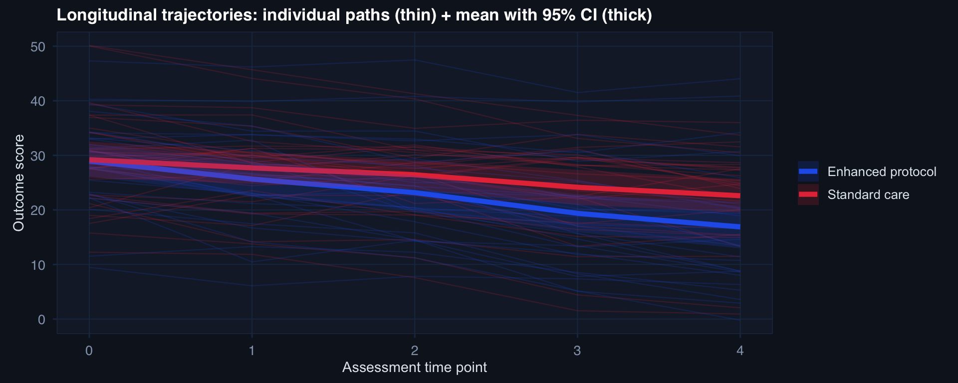
A cross-sectional study at time 4 compares endpoints. A longitudinal study sees the rate of change — and whether the groups diverge over time. These are different scientific questions.
Attrition: The Silent Threat
# Simulate: sicker patients more likely to drop out (MNAR attrition)
n <- 300; n_time <- 6
df_attr <- expand_grid(id=1:n, time=0:(n_time-1)) |>
  mutate(
    severity = rnorm(n, 30, 10)[id],
    # Higher severity → higher dropout probability each wave
    p_drop   = plogis(-3 + 0.06*severity + 0.4*time),
    dropout  = rbinom(n*n_time, 1, p_drop),
    observed = !as.logical(cummax(dropout))
  ) |>
  group_by(id) |>
  mutate(still_in = cumprod(as.integer(!dropout))) |> ungroup()

df_attr |> group_by(time) |>
  summarise(n_obs=sum(still_in==1),
            mean_sev=mean(severity[still_in==1])) |>
  pivot_longer(-time) |>
  mutate(name=recode(name, n_obs="N remaining",
                     mean_sev="Mean severity (remaining)")) |>
  ggplot(aes(time, value, color=name)) +
  geom_line(linewidth=1.2) + geom_point(size=3) +
  facet_wrap(~name, scales="free_y") +
  scale_color_manual(values=c("#e63946","#0891b2")) +
  labs(title="MNAR attrition: N drops AND remaining patients are systematically healthier",
       x="Time point", y=NULL) +
  theme_di() + theme(legend.position="none")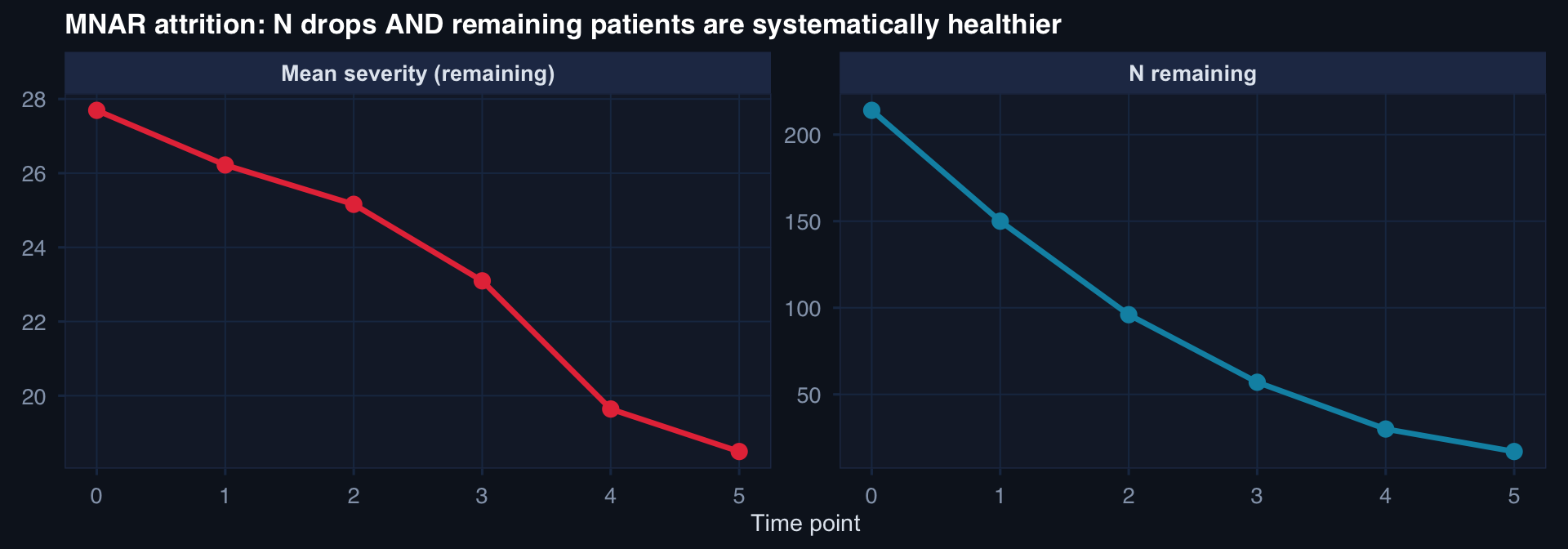
Attrition that depends on the outcome (MNAR) produces both sample loss and a biased surviving sample. Complete-case analysis will underestimate true severity trajectories. Require intent-to-treat framing and sensitivity analysis.
Power Curves: Seeing the Design Space
# Power curves for different effect sizes, two-sample t-test
n_seq <- seq(10, 300, by=5)
effects <- c(0.2, 0.5, 0.8)  # Cohen's d: small, medium, large

expand_grid(n=n_seq, d=effects) |>
  mutate(
    power = mapply(function(n, d)
      power.t.test(n=n, delta=d, sd=1, sig.level=0.05,
                   type="two.sample")$power, n, d),
    Effect = factor(paste0("d = ", d),
                    levels=c("d = 0.2","d = 0.5","d = 0.8"))
  ) |>
  ggplot(aes(n, power, color=Effect)) +
  geom_line(linewidth=1.2) +
  geom_hline(yintercept=0.80, linetype=2, color="#94a3b8") +
  scale_color_manual(values=c("#e63946","#f59e0b","#0891b2")) +
  scale_y_continuous(labels=scales::percent_format()) +
  annotate("text", x=270, y=0.83, label="80% power", color="#94a3b8", size=3.5) +
  labs(title="Power vs. sample size per group — small effects require large n",
       x="n per group", y="Power") +
  theme_di()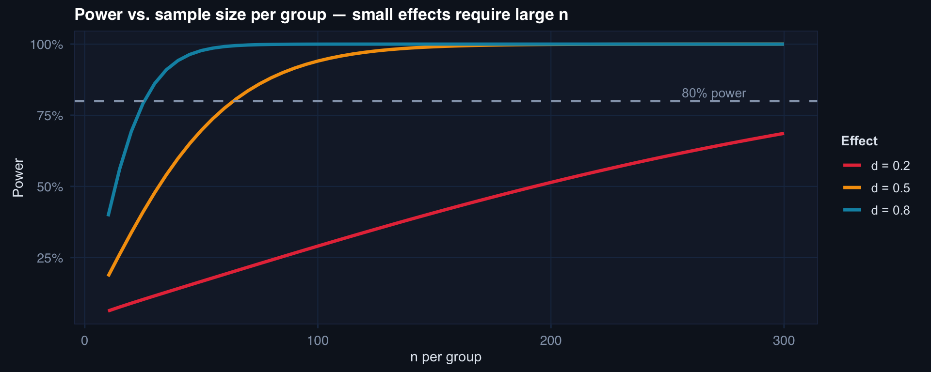
Small effect (d=0.2): needs ~400/group for 80% power. Medium (d=0.5): ~65/group. Large (d=0.8): ~26/group.
Simulation-Based Power: When Formulas Don’t Exist
# Power by simulation for a binary outcome with logistic model
sim_power <- function(n, true_or=2.0, prev=0.15, nsim=500) {
  mean(replicate(nsim, {
    trt <- rbinom(n, 1, 0.5)
    p   <- plogis(log(prev/(1-prev)) + log(true_or)*trt)
    y   <- rbinom(n, 1, p)
    tryCatch(
      coef(summary(glm(y~trt, family=binomial)))[2,"Pr(>|z|)"] < 0.05,
      error=function(e) FALSE
    )
  }))
}

n_grid <- c(50, 100, 150, 200, 300)
pwr    <- sapply(n_grid, sim_power)

tibble(n=n_grid, power=pwr) |>
  ggplot(aes(n, power)) +
  geom_line(linewidth=1.3, color="#0891b2") +
  geom_point(size=4, color="#22d3ee") +
  geom_hline(yintercept=0.80, linetype=2, color="#e63946") +
  scale_y_continuous(labels=scales::percent_format(), limits=c(0,1)) +
  labs(title="Simulation-based power: binary outcome, OR=2.0, baseline prevalence 15%",
       x="n per group", y="Empirical power (500 sims)") +
  theme_di()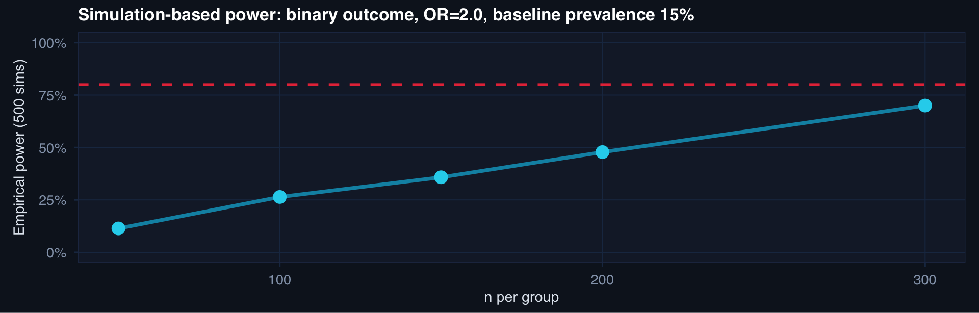
Simulation handles any design — clustered data, non-normal outcomes, survival endpoints — where closed-form formulas don’t exist.
Sensitivity Analysis for Power Inputs
# How sensitive is required n to assumptions about delta and sigma?
expand_grid(
  delta = c(0.3, 0.4, 0.5),
  sigma = c(0.8, 1.0, 1.2)
) |> mutate(
  n_required = ceiling(mapply(function(d, s)
    power.t.test(delta=d, sd=s, sig.level=0.05,
                 power=0.80, type="two.sample")$n,
    delta, sigma)),
  label = paste0("δ=", delta)
) |>
  ggplot(aes(sigma, n_required, color=label, group=label)) +
  geom_line(linewidth=1.1) +
  geom_point(size=3) +
  scale_color_manual(values=c("#e63946","#f59e0b","#0891b2")) +
  labs(title="n required for 80% power — sensitive to both effect size and variance assumptions",
       x="Assumed σ", y="Required n per group", color="Effect size (δ)") +
  theme_di()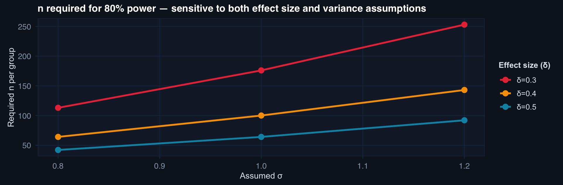
Plan for the worst case: if σ could plausibly be 20% larger than your pilot estimate, power your study for that larger σ. A sensitivity table across plausible (δ, σ) combinations belongs in every protocol.
Why Simple Randomization Sometimes Fails
# Show that simple randomization can produce temporal imbalance
set.seed(999)
n <- 60
simple_trt <- cumsum(rbinom(n, 1, 0.5) * 2 - 1)  # running balance
block_trt  <- rep(c(1,1,0,0,1,0,1,0,0,1,1,0,1,0,0,1), length.out=n)
block_balance <- cumsum(block_trt * 2 - 1)

tibble(
  enrollment = 1:n,
  Simple     = simple_trt,
  Block      = block_balance
) |> pivot_longer(-enrollment) |>
  ggplot(aes(enrollment, value, color=name)) +
  geom_line(linewidth=1.0) +
  geom_hline(yintercept=0, linetype=2, color="#94a3b8") +
  scale_color_manual(values=c("#0891b2","#e63946")) +
  labs(title="Running treatment imbalance: simple randomization drifts; block stays near 0",
       x="Patient enrolled", y="Cumulative imbalance (treated − control)", color=NULL) +
  theme_di()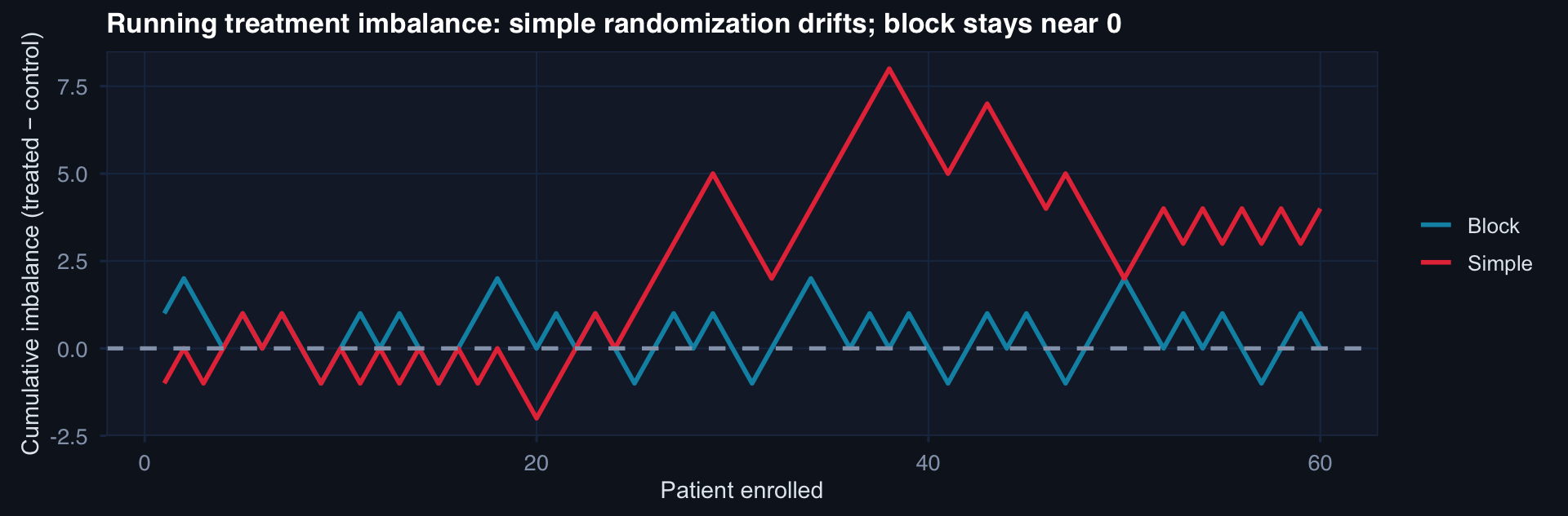
If enrollment is stopped early or interrupted, simple randomization may leave groups imbalanced. Block randomization guarantees near-equal allocation at every block boundary.
Balance Diagnostics After Randomization
n <- 200
strata <- sample(c("Blunt/Low ISS","Blunt/High ISS",
                   "Penetrating/Low ISS","Penetrating/High ISS"), n, replace=TRUE)

# Stratified block randomization (simplified: 1:1 within strata)
df_rand <- tibble(strata=strata) |>
  group_by(strata) |>
  mutate(trt=sample(rep(0:1, ceiling(n()/2))[1:n()])) |>
  ungroup() |>
  mutate(
    iss  = ifelse(grepl("High", strata), rnorm(n,38,8), rnorm(n,20,6)),
    age  = rnorm(n, 32, 12),
    sbp  = rnorm(n, 108, 22)
  )

smd <- function(x, t) abs(mean(x[t==1])-mean(x[t==0])) /
                        sqrt((var(x[t==1])+var(x[t==0]))/2)

tibble(
  Variable = c("ISS","Age","SBP"),
  SMD = c(smd(df_rand$iss, df_rand$trt),
          smd(df_rand$age, df_rand$trt),
          smd(df_rand$sbp, df_rand$trt))
) |>
  ggplot(aes(SMD, reorder(Variable, -SMD))) +
  geom_col(fill="#0891b2", alpha=0.85, width=0.5) +
  geom_vline(xintercept=0.1, linetype=2, color="#e63946") +
  labs(title="Post-randomization balance check: all SMD < 0.10 target",
       x="Standardized Mean Difference", y=NULL) +
  theme_di()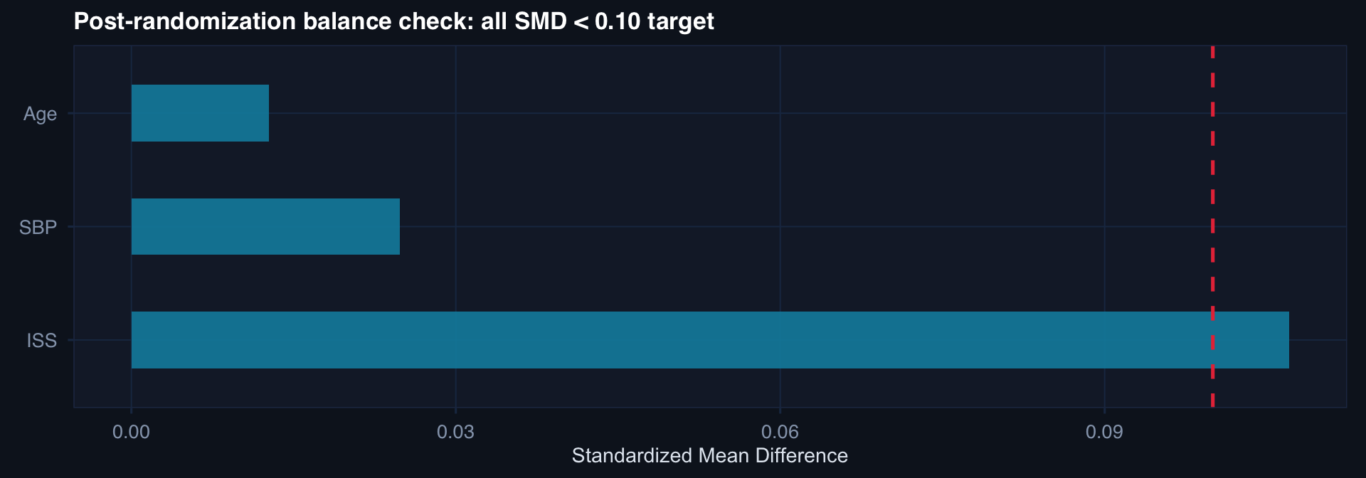
Always report a Table 1 with SMD — not p-values. In a randomized trial, any imbalance is due to chance alone, not confounding. The question is magnitude, not significance.