# Model A: high AUC, badly calibrated (overconfident at high risk)
# Model B: lower AUC, well calibrated
n <- 1000
set.seed(42)
true_p <- rbeta(n, 1.5, 8)  # true risk: mostly low, some high
y      <- rbinom(n, 1, true_p)

# Model A: discriminates well, but systematically overestimates at high end
pred_a <- pmin(plogis(qlogis(true_p) + rnorm(n, 0.5, 0.8)), 0.99)
# Model B: slightly less discriminating, well calibrated
pred_b <- plogis(qlogis(true_p) + rnorm(n, 0, 1.1))

auc_a <- as.numeric(pROC::auc(pROC::roc(y, pred_a, quiet=TRUE)))
auc_b <- as.numeric(pROC::auc(pROC::roc(y, pred_b, quiet=TRUE)))

bind_rows(
  tibble(model="A (AUC=.84, miscalibrated)", pred=pred_a, y=y),
  tibble(model="B (AUC=.79, calibrated)",    pred=pred_b, y=y)
) |>
  mutate(decile=ntile(pred, 10)) |>
  group_by(model, decile) |>
  summarise(pred_mean=mean(pred), obs=mean(y), .groups="drop") |>
  ggplot(aes(pred_mean, obs, color=model)) +
  geom_abline(linetype=2, color="#64748b") +
  geom_line(linewidth=1) + geom_point(size=3) +
  scale_color_manual(values=c("#e63946","#0891b2")) +
  labs(title="Model A has higher AUC but is miscalibrated — Model B is safer for decisions",
       x="Mean predicted risk", y="Observed event rate", color=NULL) +
theme_di()Registry Foundations: Why Models Fail & How to Analyze Honestly
Trauma Registry Analytics — Lecture 1 of 5
2026-01-01
The Myth of “Good Performance”
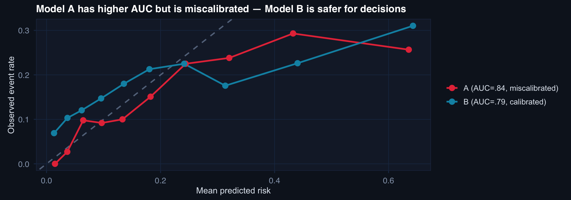
AUC tells you about ranking. Calibration tells you whether the numbers mean anything. A model that says 40% risk when the true risk is 15% will cause harm — regardless of its AUC.
Dataset Shift: The Default Condition
# Train on 2018-2021 DoDTR analog; test on 2022-2024 (protocol change + population shift)
n_train <- 600; n_test <- 300

df_train <- tibble(
  iss   = rnorm(n_train, 26, 11),
  era   = "Train (2018–21)",
  died  = rbinom(n_train, 1, plogis(-3.5 + 0.08*iss))
)
df_test <- tibble(
  iss   = rnorm(n_test, 31, 13),   # higher severity in later era
  era   = "Test (2022–24)",
  died  = rbinom(n_test, 1, plogis(-4.0 + 0.08*iss))  # improved care
)

bind_rows(df_train, df_test) |>
  ggplot(aes(iss, fill=era, color=era)) +
  geom_density(alpha=0.4, linewidth=0.8) +
  scale_fill_manual(values=c("#2563eb","#e63946")) +
  scale_color_manual(values=c("#2563eb","#e63946")) +
  labs(title="ISS distribution shift between training and test eras — model trained on blue, deployed to red",
       x="ISS", y="Density", fill=NULL, color=NULL) +
  theme_di()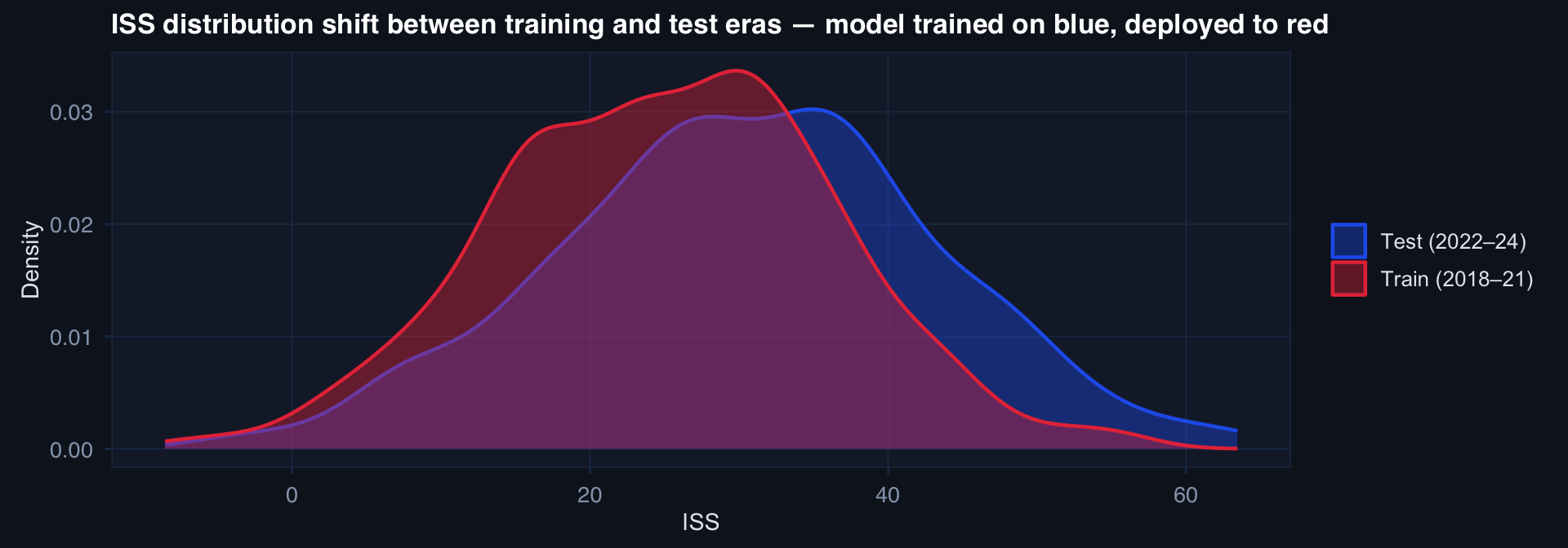
A model trained on the blue distribution will be systematically miscalibrated on the red population — not because the model is wrong, but because the world changed.
Time Is the Most Abused Variable
# Simulate: outcome rates changing over time (improving care + worsening case mix)
months <- seq(as.Date("2019-01-01"), as.Date("2024-12-01"), by="month")
n_m <- length(months)

df_time <- tibble(
  month      = months,
  iss_mean   = 24 + 0.12 * seq_len(n_m) + rnorm(n_m, 0, 1.5),   # worsening case mix
  care_effect = -0.008 * seq_len(n_m),                              # improving protocols
  mortality   = plogis(-2.5 + 0.04*iss_mean + care_effect + rnorm(n_m, 0, 0.15))
)

df_time |>
  pivot_longer(c(iss_mean, mortality)) |>
  mutate(name=recode(name, iss_mean="Mean ISS (case mix)",
                     mortality="Observed mortality rate")) |>
  ggplot(aes(month, value, color=name)) +
  geom_line(linewidth=1.1) +
  geom_smooth(method="loess", se=FALSE, linewidth=0.7, linetype=3) +
  facet_wrap(~name, scales="free_y") +
  scale_color_manual(values=c("#e63946","#0891b2")) +
  labs(title="Simultaneous case-mix worsening and care improvement — naive trend is misleading",
       x=NULL, y=NULL) +
  theme_di() + theme(legend.position="none")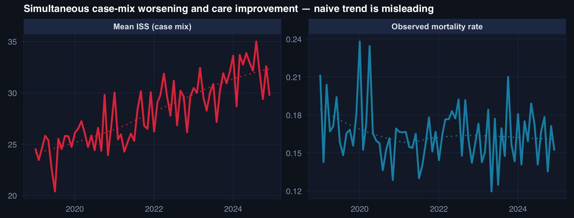
A rising mortality trend may mean care is getting worse — or that cases are getting harder. Disentangling requires risk-adjusted analysis over time, not raw trend lines.