Modeling Philosophy: Bayesian Thinking, Beyond p-Values & Hierarchical Models

Trauma Registry Analytics — Lecture 2 of 5

Jonathan D. Stallings, PhD, MS

Data InDeed | dataindeed.org

2026-01-01

p < 0.05 tells you that something happened. It does not tell you what to do about it.

What You’ll Learn Today

Post 03 Bayesian Thinking

  • Priors as transparency
  • Posterior distributions
  • Credible vs. confidence intervals
  • Decision-focused outputs

Post 06 Beyond p-Values

  • What p < 0.05 actually answers
  • Effect size vs. significance
  • Better questions, better metrics
  • When significance causes harm

Post 07 Hierarchical Models

  • The independence violation
  • Partial pooling
  • The minimal multilevel model
  • When hierarchy changes the answer

Part 1

Bayesian Thinking for Clinicians

Updating beliefs with evidence

The Bayesian Equation — In Clinical Language

\[P(\theta \mid \text{data}) \propto P(\text{data} \mid \theta) \cdot P(\theta)\]

PosteriorLikelihood × Prior

“What I believe after seeing the data = what the data supports × what I believed before.”

Why this matches clinical reasoning:

A trauma surgeon with 15 years of experience seeing a GCS-3 patient doesn’t start from a blank slate. They update their prior beliefs (from thousands of similar cases) with the new information.

That’s Bayesian reasoning — it’s what good clinicians already do.

The frequentist alternative: pretend you have no prior information, then report whether the data is “surprising” under a null hypothesis you don’t actually believe.

Prior is not bias — it’s transparency.

A non-informative prior says “I have no prior information.” That’s almost never true.

A weakly informative prior says “I expect effects in this plausible range, based on similar studies.” That’s honest.

A strong prior should require strong justification — and be subjected to sensitivity analysis.

Posterior Uncertainty vs. Point Estimates

# Beta-Binomial: estimating mortality rate with prior knowledge
# Prior: Beta(3, 17) = prior belief of ~15% mortality from previous theater
alpha_prior <- 3; beta_prior <- 17

# Observed: 14 deaths in 60 patients
deaths <- 14; total <- 60
alpha_post <- alpha_prior + deaths
beta_post  <- beta_prior + (total - deaths)

x <- seq(0, 0.6, length.out=300)
bind_rows(
  tibble(x=x, dens=dbeta(x, alpha_prior, beta_prior),
         dist="Prior Beta(3,17)\n[~15% belief]"),
  tibble(x=x, dens=dbeta(x, alpha_post,  beta_post),
         dist="Posterior Beta(17,63)\n[14/60 observed]")
) |>
  ggplot(aes(x, dens, fill=dist, color=dist)) +
  geom_area(alpha=0.35, position="identity") +
  geom_line(linewidth=1.2) +
  geom_vline(xintercept=alpha_post/(alpha_post+beta_post),
             linetype=2, color="#f59e0b") +
  scale_fill_manual(values=c("#2563eb","#e63946")) +
  scale_color_manual(values=c("#2563eb","#e63946")) +
  annotate("text", x=0.29, y=8, label=paste0("Posterior mean\n",
    round(alpha_post/(alpha_post+beta_post)*100,1),"%"),
    color="#f59e0b", size=3.5) +
  labs(title="Bayesian update: prior belief + 14/60 data → posterior distribution over mortality rate",
       x="Mortality rate θ", y="Density", fill=NULL, color=NULL) +
  theme_di()

The posterior is a full distribution — not a point estimate. It quantifies uncertainty honestly. The 95% credible interval contains the true value with 95% probability (unlike a confidence interval, which doesn’t quite say that).

Credible Intervals vs. Confidence Intervals

Credible Interval (Bayesian) Confidence Interval (Frequentist)
Statement “P(θ in [a,b] | data) = 95%” “95% of such intervals contain θ”
What it says Probability the parameter is here Property of the procedure, not this interval
What clinicians hear What they want Also what they want (but shouldn’t)
Requires prior Yes — transparently No — implicitly flat prior

The practical difference matters most for small n:

With n=30 and 3 events, the frequentist CI may be numerically unstable. The Bayesian credible interval incorporates prior information to produce a stable, interpretable interval — if the prior is honest.

Part 2

Beyond Statistical Significance

What p < 0.05 cannot answer

What p < 0.05 Actually Answers

p-value = P(data this extreme or more | H₀ is exactly true)

It does not answer:

  • P(H₀ is true | data) — that’s Bayesian
  • Whether the effect is clinically meaningful
  • Whether the finding will replicate
  • Whether you should change practice
# Same effect, different n → different p-value
set.seed(77)
effect <- 0.3  # small but real effect

results <- tibble(n = c(30, 100, 300, 1000, 5000)) |>
  mutate(
    p_val = sapply(n, function(n) {
      x <- rnorm(n, effect, 1); y <- rnorm(n, 0, 1)
      t.test(x, y)$p.value
    }),
    sig = p_val < 0.05
  )

ggplot(results, aes(n, p_val, color=sig)) +
  geom_hline(yintercept=0.05, linetype=2, color="#94a3b8") +
  geom_point(size=5) +
  geom_line(color="#64748b", linewidth=0.5) +
  scale_color_manual(values=c("#e63946","#0891b2"),
                     labels=c("p ≥ 0.05","p < 0.05")) +
  scale_x_log10() +
  annotate("text", x=4000, y=0.08, label="α = 0.05", color="#94a3b8", size=3.5) +
  labs(title="True effect d=0.3 becomes 'significant' only when n is large enough — the effect didn't change",
       x="Sample size (log scale)", y="p-value", color=NULL) +
  theme_di()

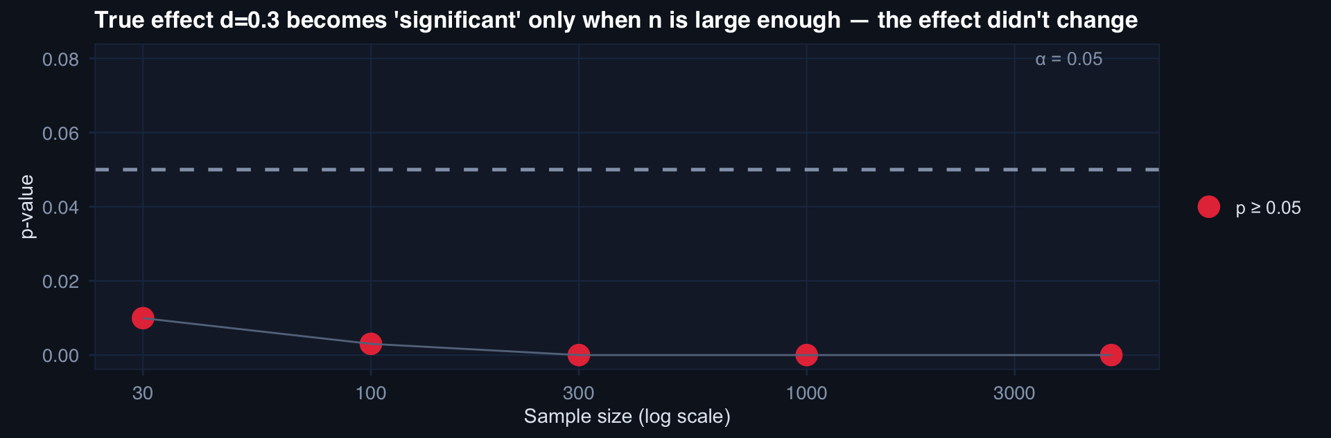
With n=5000, even a trivially small effect is “significant.” Sample size turns anything into a discovery.

Better Questions for Clinical Decision-Making

Replace this:

“Is the treatment statistically significantly better?”

With these:

  1. What is the magnitude of the effect, with honest uncertainty?
  2. Is the effect clinically meaningful — above the minimum important difference?
  3. What is the probability the effect exceeds a decision threshold?
  4. How robust is the conclusion to different assumptions?
  5. What would it take to overturn this finding?

Report instead of p-values:

Effect size + CI (absolute, not just relative)

Minimum clinically important difference (MCID)

P(effect > MCID) — Bayesian

E-value — sensitivity to confounding

Number needed to treat (NNT)

Part 3

Hierarchical Models

When independence is the violated assumption, not the missing variable

The Silence of Flat Models

# Simulate clustered trauma data: patients within facilities
n_facilities <- 15; n_per <- 25
facility_effects <- rnorm(n_facilities, 0, 0.6)

df_hier <- expand_grid(
  facility = 1:n_facilities,
  patient  = 1:n_per
) |> mutate(
  u_fac    = facility_effects[facility],
  iss      = rnorm(n(), 28, 10),
  died     = rbinom(n(), 1, plogis(-3 + 0.07*iss + u_fac))
)

# Mortality rate by facility
fac_rates <- df_hier |>
  group_by(facility) |>
  summarise(rate=mean(died), n=n(), mean_iss=mean(iss))

ggplot(fac_rates, aes(reorder(factor(facility), rate), rate)) +
  geom_col(fill="#0891b2", alpha=0.8) +
  geom_hline(yintercept=mean(fac_rates$rate), linetype=2, color="#e63946") +
  labs(title="Mortality varies substantially across facilities — ignoring this inflates false positives",
       x="Facility (sorted by mortality rate)", y="Observed mortality rate") +
  theme_di() + theme(axis.text.x=element_blank())

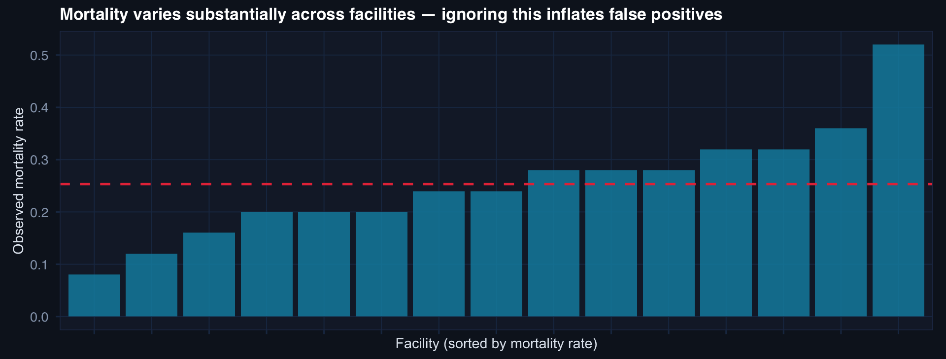
ICC = 0.10 here. This means 10% of outcome variance is explained by facility membership alone. Every patient-level model that ignores facility is pooling patients across structurally different care contexts — as if a Role 2 facility in a contested environment and a Role 4 stateside hospital were identical.

Partial Pooling: The Core Idea

# Compare: no pooling (raw rates) vs. partial pooling (shrinkage estimate)
fac_rates <- fac_rates |>
  mutate(
    grand_mean    = mean(rate),
    # Shrinkage toward grand mean based on n
    shrinkage     = n / (n + 10),
    partial_pool  = shrinkage * rate + (1 - shrinkage) * grand_mean
  )

fac_rates |>
  pivot_longer(c(rate, partial_pool)) |>
  mutate(name=recode(name, rate="No pooling (raw)",
                     partial_pool="Partial pooling (shrinkage)")) |>
  ggplot(aes(reorder(factor(facility), value), value, color=name, group=name)) +
  geom_point(size=3) +
  geom_line(alpha=0.5) +
  geom_hline(yintercept=mean(fac_rates$rate), linetype=2, color="#94a3b8") +
  scale_color_manual(values=c("#e63946","#0891b2")) +
  labs(title="Partial pooling shrinks extreme estimates toward the grand mean — proportional to small n",
       x="Facility", y="Mortality rate estimate", color=NULL) +
  theme_di() + theme(axis.text.x=element_blank())

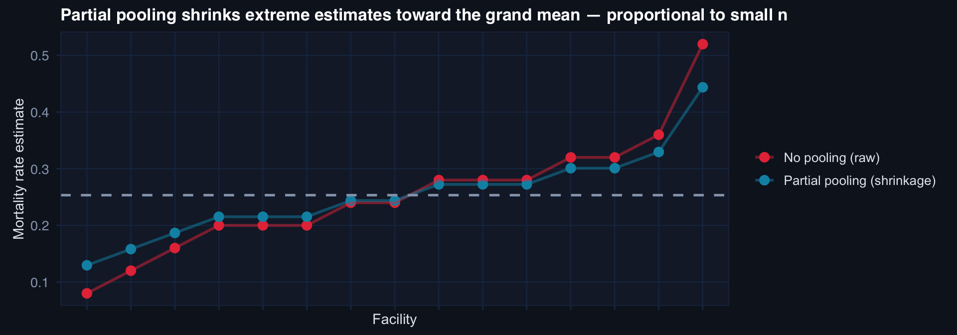
Small facilities get shrunk more — their estimates are less stable. Large facilities stay near their raw rate — their data is informative. This is automatically appropriate weighting, not ad hoc adjustment.

The Minimal Hierarchical Model in R

library(lme4)

# Random intercept model: patients within facilities
fit_flat  <- glm(died ~ iss, data=df_hier, family=binomial)
fit_hier  <- glmer(died ~ iss + (1 | facility), data=df_hier,
                   family=binomial)

# Compare facility-level variance captured
cat("Flat model — no facility variance captured\n")
Flat model — no facility variance captured
cat("Residual deviance:", deviance(fit_flat), "\n\n")
Residual deviance: 402.3553 
cat("Hierarchical model — facility random intercept\n")
Hierarchical model — facility random intercept
VarCorr(fit_hier)
 Groups   Name        Std.Dev.
 facility (Intercept) 0.13452 
cat("ISS coefficient (flat):  ", round(coef(fit_flat)["iss"], 4), "\n")
ISS coefficient (flat):   0.0558 
cat("ISS coefficient (hier):  ", round(fixef(fit_hier)["iss"], 4), "\n")
ISS coefficient (hier):   0.0555 

When hierarchy changes the answer: If facility-level variation is large (ICC > 0.05), the flat model’s standard errors are too small — significance is inflated. Any p-value from a flat model on clustered registry data should be treated with suspicion.

Lecture 2 — Key Takeaways

Bayesian Thinking

  • Prior = transparency about what you knew before data
  • Posterior = full distribution, not a point estimate
  • Credible interval: P(θ ∈ [a,b] | data) — clinically interpretable
  • Decision-focused: P(effect > threshold), not just “significant”

Beyond p-Values

  • p-value answers: data surprising under H₀? Not: is H₀ false?
  • Large n makes everything significant — effect size is what matters
  • Report: magnitude + CI + MCID comparison + sensitivity

Hierarchical Models

  • Independence is violated by default in registry data
  • ICC > 0.05 → flat model SEs are anti-conservative
  • Partial pooling: shrinkage toward grand mean, proportional to n
  • glmer(outcome ~ predictors + (1 | facility)) is the minimum
  • Random slopes needed when treatment effects vary by facility

The meta-lesson: These three ideas — Bayesian updating, effect-size thinking, and hierarchical structure — are not advanced methods. They are the correct default for registry analytics. The flat frequentist model is the special case, not the standard.

Coming Up: Lecture 3

Missing Data Deep Dive: Strategies, Hierarchical Missingness & MNAR

Posts 04, 14 & 15:

  • Missing data strategies — mechanism thinking, imputation, sensitivity
  • Missing data in hierarchical models — why structure changes the problem
  • MNAR sensitivity analysis — delta adjustment, bounding, reviewer-ready reporting