n <- 500
df_reg <- tibble(
  iss       = rnorm(n, 28, 12),
  sbp       = rnorm(n, 108, 24),
  treatment = rbinom(n, 1, 0.45)
) |> mutate(
  # Lactate missing more for high-ISS, low-SBP patients (sicker = less documented)
  p_miss_lactate = plogis(-1.5 + 0.06*iss - 0.02*sbp),
  lactate_miss   = rbinom(n, 1, p_miss_lactate),
  # GCS missing more in penetrating/high mechanism injuries
  p_miss_gcs     = plogis(-2 + 0.04*iss),
  gcs_miss       = rbinom(n, 1, p_miss_gcs)
)

df_reg |>
  group_by(iss_group = cut(iss, breaks=c(0,15,25,35,75),
                           labels=c("<15","15–25","25–35","35+"))) |>
  summarise(across(c(lactate_miss, gcs_miss), mean), .groups="drop") |>
  pivot_longer(-iss_group) |>
  mutate(name=recode(name, lactate_miss="Lactate missing",
                     gcs_miss="GCS missing")) |>
  ggplot(aes(iss_group, value, fill=name)) +
  geom_col(position="dodge", alpha=0.85) +
  scale_fill_manual(values=c("#0891b2","#e63946")) +
  scale_y_continuous(labels=scales::percent_format()) +
  labs(title="Missingness rate rises with severity — this is MAR, not MCAR",
       x="ISS group", y="% missing", fill=NULL) +
theme_di()Missing Data Deep Dive: Strategies, Hierarchy & MNAR
Trauma Registry Analytics — Lecture 3 of 5
2026-01-01
Missingness as a Variable, Not a Nuisance
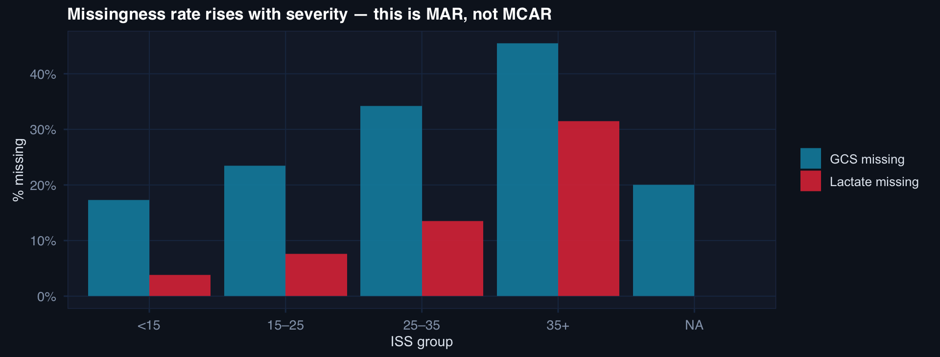
The missingness pattern is data about data quality under pressure. High-ISS patients have more missing labs because they were too unstable for a full workup — not because data was lost randomly.
Visualizing Missingness First
# Missingness pattern matrix (simplified naniar-style)
vars <- c("lactate","gcs","sbp_arrival","mechanism","transport_time","blood_units")
n_show <- 80

set.seed(9)
miss_mat <- tibble(patient = 1:n_show) |>
  mutate(
    lactate       = rbinom(n_show, 1, 0.32),
    gcs           = rbinom(n_show, 1, 0.18),
    sbp_arrival   = rbinom(n_show, 1, 0.08),
    mechanism     = rbinom(n_show, 1, 0.04),
    transport_time= rbinom(n_show, 1, 0.22),
    blood_units   = rbinom(n_show, 1, 0.15)
  )

miss_mat |>
  pivot_longer(-patient, names_to="variable", values_to="missing") |>
  ggplot(aes(variable, factor(patient), fill=factor(missing))) +
  geom_tile(color="#0f1724", linewidth=0.3) +
  scale_fill_manual(values=c("#162032","#e63946"),
                    labels=c("Observed","Missing")) +
  labs(title="Missingness pattern heatmap — look for co-missing variables and patient clusters",
       x=NULL, y="Patient", fill=NULL) +
  theme_di() + theme(axis.text.y=element_blank(),
                     axis.ticks.y=element_blank())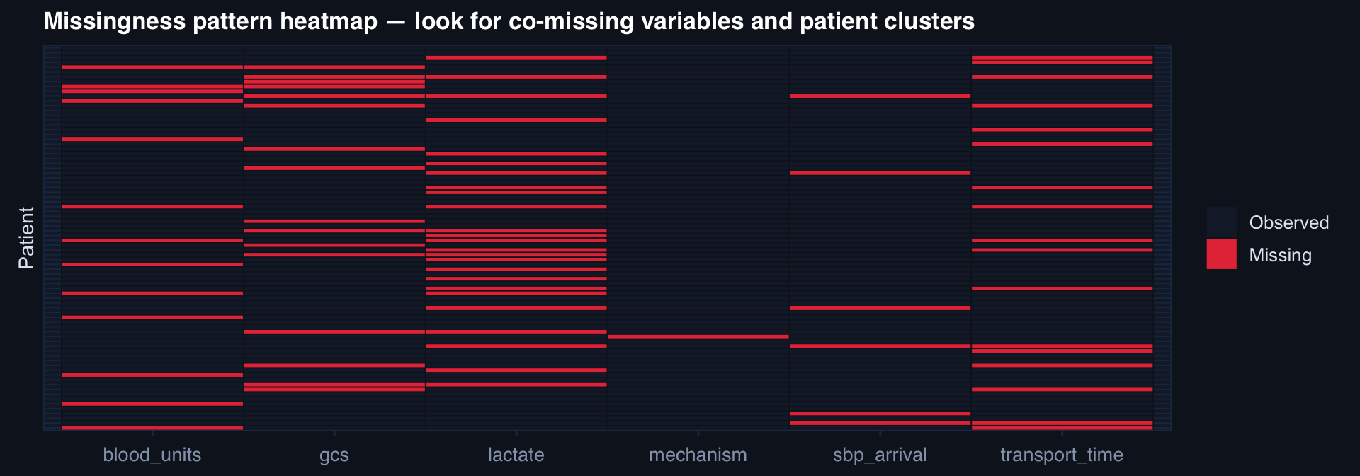
Co-missingness patterns reveal mechanism: lactate and transport time missing together suggests prehospital-phase data gaps, not random documentation failure.
Why Mean Imputation Is Worse Than Complete-Case
n <- 400
sbp_true <- rnorm(n, 108, 28)
miss_idx  <- which(sbp_true < 90 | runif(n) > 0.75)  # MNAR: low SBP more missing

sbp_cc    <- sbp_true[-miss_idx]           # complete case
sbp_mean  <- sbp_true; sbp_mean[miss_idx] <- mean(sbp_true[-miss_idx])

tibble(
  Approach = c(rep("Complete-case", length(sbp_cc)),
               rep("Mean-imputed",  length(sbp_mean))),
  SBP = c(sbp_cc, sbp_mean)
) |>
  ggplot(aes(SBP, fill=Approach, color=Approach)) +
  geom_density(alpha=0.4, linewidth=0.8) +
  geom_vline(xintercept=mean(sbp_true), linetype=2, color="#94a3b8") +
  scale_fill_manual(values=c("#2563eb","#e63946")) +
  scale_color_manual(values=c("#2563eb","#e63946")) +
  labs(title="Mean imputation removes the left tail (low SBP = high-risk) — the clinically critical range",
       x="SBP at arrival", y="Density", fill=NULL, color=NULL) +
  theme_di()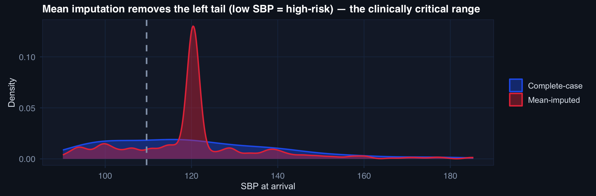
Mean imputation in MNAR settings actively removes the information you care most about — the physiologic extremes that drive mortality. It produces false precision and wrong estimates simultaneously.
Group-Structured Missingness Pattern
n_fac <- 12; n_per <- 40
fac_miss_rates <- c(rep(0.08, 4), rep(0.25, 4), rep(0.45, 4))  # low/mid/high miss

df_hmiss <- expand_grid(facility=1:n_fac, patient=1:n_per) |>
  mutate(
    role     = case_when(facility <= 4 ~ "Role 4", facility <= 8 ~ "Role 3",
                         TRUE ~ "Role 2"),
    p_miss   = fac_miss_rates[facility],
    lactate_miss = rbinom(n(), 1, p_miss),
    iss      = rnorm(n(), ifelse(role=="Role 2", 35, ifelse(role=="Role 3", 28, 22)), 10)
  )

df_hmiss |>
  group_by(facility, role) |>
  summarise(miss_rate=mean(lactate_miss), mean_iss=mean(iss), .groups="drop") |>
  ggplot(aes(mean_iss, miss_rate, color=role, label=facility)) +
  geom_point(size=5) +
  ggrepel::geom_text_repel(size=3, color="#e2e8f0") +
  scale_color_manual(values=c("#e63946","#f59e0b","#0891b2")) +
  scale_y_continuous(labels=scales::percent_format()) +
  labs(title="Higher-acuity facilities (Role 2) have both higher ISS and higher missingness",
       x="Mean ISS", y="Lactate missing rate", color="Role of care") +
  theme_di()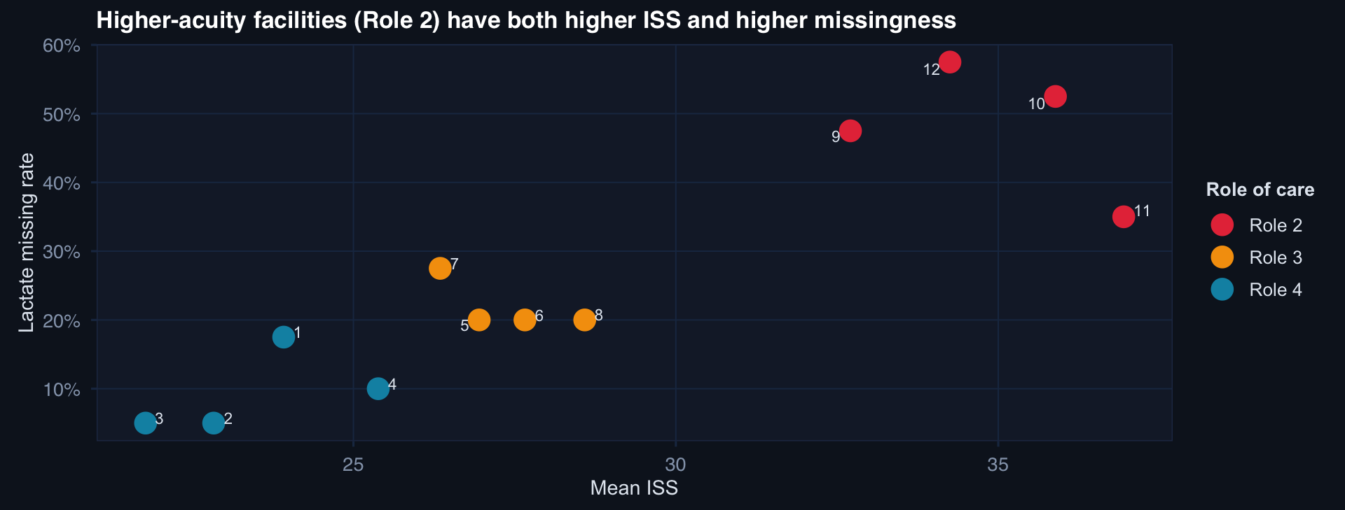
Missingness and severity are correlated at the facility level. Any imputation model that ignores facility will systematically understate severity for high-missingness, high-acuity sites.
Delta Adjustment in the Registry Context
# Scenario: lactate missing for sicker patients
# True effect of early intervention on mortality
n <- 500
df_mnar <- tibble(
  iss       = rnorm(n, 28, 12),
  early_tx  = rbinom(n, 1, plogis(-0.5 + 0.02*iss)),
  # Lactate: higher in sicker; missing if lactate > 4 OR random (MNAR)
  lactate   = 1.5 + 0.08*iss + rnorm(n, 0, 1.2),
  lac_obs   = ifelse(lactate > 4 | runif(n) > 0.7, NA, lactate),
  died      = rbinom(n, 1, plogis(-3 + 0.07*iss - 1.2*early_tx + 0.2*lactate))
)

# Impute at delta increments above observed mean
deltas <- seq(0, 3, by=0.5)
effects <- sapply(deltas, function(d) {
  df_imp <- df_mnar |>
    mutate(lac_imp = ifelse(is.na(lac_obs),
                            mean(lac_obs, na.rm=TRUE) + d, lac_obs))
  coef(glm(died ~ early_tx + iss + lac_imp, data=df_imp, family=binomial))["early_tx"]
})

tibble(delta=deltas, log_or=effects) |>
  ggplot(aes(delta, log_or)) +
  geom_line(linewidth=1.3, color="#0891b2") +
  geom_point(size=4, color="#22d3ee") +
  geom_hline(yintercept=0, linetype=2, color="#e63946") +
  labs(title="MNAR sensitivity: effect of early treatment as missing lactate is assumed higher",
       x="δ added to missing lactate values (mmol/L above observed mean)",
       y="Log-OR for early treatment") +
  theme_di()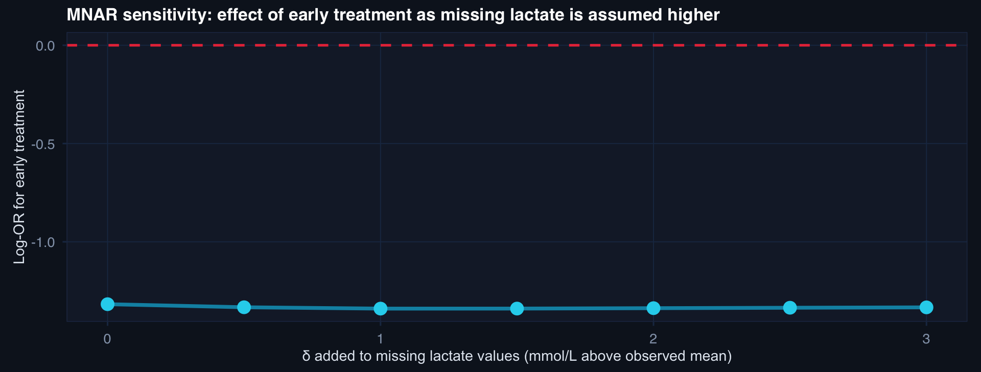
The effect remains protective (negative log-OR) across δ = 0 to 2.5. The tipping point is beyond δ = 3 — clinically implausible for lactate.