library(dplyr)
library(tibble)
library(ggplot2)

n <- 1000

iv_df <- tibble::tibble(
  z = rbinom(n, size = 1, prob = 0.5),   # encouragement / instrument
  u = rnorm(n, mean = 0, sd = 1),        # unmeasured confounder
  x = rnorm(n, mean = 0, sd = 1)         # measured covariate
) |>
  dplyr::mutate(
    treatment = 0.8 * z + 0.9 * u + 0.5 * x + rnorm(n, 0, 1),
    outcome = 2.5 * treatment + 1.2 * u + 0.6 * x + rnorm(n, 0, 1)
)Instrumental Variables: Uncovering Hidden Causes in ML
Advanced Statistics
A practical introduction to instrumental variables, endogeneity, two-stage least squares, and causal identification under unmeasured confounding.
Executive Summary
One of the hardest problems in causal inference is unmeasured confounding (Lousdal 2018; Greenland 2000).
Even after adjusting for observed covariates, the treatment and outcome may still be linked through factors we did not measure well — or did not measure at all.
That is where instrumental variable (IV) methods become important.
An instrumental variable is a variable that helps shift treatment exposure but does not affect the outcome except through that treatment. If such a variable exists and the assumptions are plausible, IV methods can recover causal information even when standard adjustment fails because of hidden confounding (Angrist et al. 1996; Lousdal 2018).
This matters in real-world evidence and observational healthcare data, where treatment assignment is often influenced by factors such as:
- adherence,
- physician preference,
- site practices,
- access barriers,
- and patient motivation.
This post introduces:
- what makes a valid instrument,
- why IV methods are useful,
- two-stage least squares (2SLS),
- endogeneity testing with the Hausman idea,
- and a simple treatment-adherence style simulation.
Instrumental variables matter because when the treatment comparison is biased by hidden confounding, a credible external source of treatment variation can sometimes recover causal leverage.
Instrumental Variables Begin Where Standard Adjustment Breaks Down
Many causal methods assume that once we adjust for observed covariates, treatment assignment is as good as random.
That is the core logic behind regression adjustment, matching, and propensity scores.
But what if that is not true?
What if important confounders remain unmeasured?
Examples include:
- motivation,
- adherence tendency,
- physician concern,
- subtle severity signals,
- family support,
- or access constraints.
In those settings, conventional observational comparisons remain biased.
Instrumental variable methods are designed for exactly this problem: they try to isolate variation in treatment that is less contaminated by unmeasured confounding.
A Valid Instrument Must Satisfy Three Core Ideas
An instrumental variable is not just any predictor of treatment.
A useful instrument must satisfy several strong conditions (Lousdal 2018).
Relevance
The instrument must be associated with treatment.
\[ Z \rightarrow T \]
If the instrument does not meaningfully shift treatment, it cannot help identify the effect.
Exclusion Restriction
The instrument should affect the outcome only through treatment.
That means no direct path from the instrument to the outcome except through treatment.
Independence
The instrument should be independent of unmeasured confounders affecting the outcome.
This is what gives the IV its causal leverage.
These assumptions are strong. IV analysis is powerful only when the instrument is genuinely credible.
The Main Idea Is to Use External Variation in Treatment
The intuition behind IV is simple:
- some part of treatment variation is confounded,
- but another part may be driven by an external factor that is more plausibly exogenous.
If we can isolate the external part, we can use that variation to learn about the treatment effect.
This is why instruments are often variables like:
- geographic prescribing variation,
- random encouragement,
- policy eligibility thresholds,
- physician preference,
- site-level practice tendencies,
- or treatment assignment nudges.
These are not perfect automatically. But when plausible, they provide a way to separate treatment variation from confounding variation.
A Biostats-Style Adherence Example Makes the Problem Concrete
To make the idea practical, we will simulate a treatment-adherence style example.
Suppose we are interested in the effect of actual treatment receipt on an outcome, but actual receipt is confounded by an unmeasured factor such as motivation or engagement.
We will use a randomized-style encouragement variable as an instrument.
Here:
zaffects treatment,uaffects both treatment and outcome,- and
uis unmeasured in the causal analysis.
That means ordinary regression of outcome on treatment will be biased.
Ordinary Regression Is Biased Under Endogeneity
Before using IV, let us fit the naïve regression model that ignores the hidden confounder.
fit_ols <- lm(outcome ~ treatment + x, data = iv_df)

summary(fit_ols)$coefficients
Estimate Std. Error t value Pr(>|t|)
(Intercept) -0.3009745 0.04375856 -6.878072 1.069576e-11
treatment 3.0411360 0.02915831 104.297399 0.000000e+00
x 0.2767749 0.04564646 6.063447 1.888297e-09Because treatment is correlated with the unmeasured confounder u, the OLS treatment coefficient is biased.
This is the core problem of endogeneity:
the treatment variable is correlated with the error term in the outcome model.
That breaks a key regression assumption.
Endogeneity Is What IV Methods Are Designed to Address
A variable is endogenous when it is correlated with the outcome error term.
This can happen because of:
- omitted variables,
- reverse causation,
- measurement error,
- or selection processes.
In our example, treatment is endogenous because the hidden variable u affects both treatment and outcome.
This is why OLS cannot isolate the treatment effect properly.
IV methods try to solve this by replacing the problematic treatment variation with instrument-driven variation.
That is the central identification move.
Two-Stage Least Squares Implements the IV Logic
The most common linear IV estimator is two-stage least squares (2SLS).
The logic is:
Stage 1
Regress treatment on the instrument and observed covariates.
\[ T = \alpha_0 + \alpha_1 Z + \alpha_2 X + \varepsilon \]
This extracts the part of treatment explained by the instrument.
Stage 2
Regress outcome on the predicted treatment from Stage 1 and the observed covariates.
\[ Y = \beta_0 + \beta_1 \hat{T} + \beta_2 X + \eta \]
This uses only the instrument-driven component of treatment to estimate the causal effect.
That is why 2SLS is the classical implementation of IV estimation.
The First Stage Tells Us Whether the Instrument Is Relevant
Let us fit the first-stage model.
fit_stage1 <- lm(treatment ~ z + x, data = iv_df)

summary(fit_stage1)$coefficients
Estimate Std. Error t value Pr(>|t|)
(Intercept) 0.1221682 0.06099715 2.002850 4.546372e-02
z 0.6911413 0.08797409 7.856192 1.021184e-14
x 0.5442339 0.04502838 12.086464 1.754490e-31The coefficient for z should be meaningfully different from zero if the instrument is relevant.
This is important because weak instruments create unstable and unreliable IV estimates.
A valid instrument must not only satisfy exclusion and independence ideas. It must also actually move treatment.
That is why the first-stage association matters so much.
Visualizing the Instrument–Treatment Relationship Helps
A simple plot can help show instrument relevance.
iv_df |>
  dplyr::group_by(z) |>
  dplyr::summarise(
    mean_treatment = mean(treatment),
    .groups = "drop"
  ) |>
  ggplot2::ggplot(ggplot2::aes(x = factor(z), y = mean_treatment)) +
  ggplot2::geom_col() +
  ggplot2::labs(
    title = "Mean Treatment by Instrument Level",
    x = "Instrument (z)",
    y = "Mean Treatment"
  ) +
  ggplot2::theme_minimal()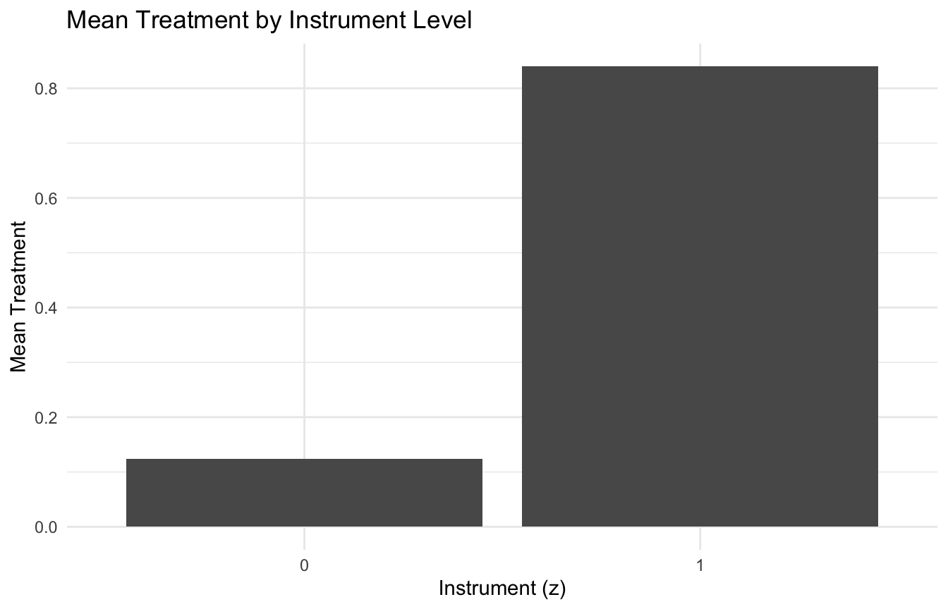
This is a simple visual reminder that the instrument must create meaningful treatment variation.
Manual Two-Stage Least Squares Makes the Mechanics Visible
We can implement the two stages manually to show the mechanics.
iv_df <- iv_df |>
  dplyr::mutate(
    treatment_hat = predict(fit_stage1)
  )

fit_stage2_manual <- lm(outcome ~ treatment_hat + x, data = iv_df)

summary(fit_stage2_manual)$coefficients
Estimate Std. Error t value Pr(>|t|)
(Intercept) 0.05132355 0.2343204 0.2190315 8.266704e-01
treatment_hat 2.26584009 0.4105580 5.5189283 4.348245e-08
x 0.70512497 0.2693232 2.6181371 8.975163e-03This gives the intuitive structure of 2SLS.
In practice, analysts usually use dedicated IV estimation functions rather than manual substitution, because the standard errors need to account properly for the two-stage estimation process.
But the manual version is excellent for understanding the logic.
Proper 2SLS Estimation Uses an IV Estimator, Not Just Manual Plug-In
For real estimation, a dedicated IV routine is preferred.
In R, a common tool is ivreg() from the AER package.
required_pkgs <- c("AER")
missing_pkgs <- required_pkgs[
  !vapply(required_pkgs, requireNamespace, logical(1), quietly = TRUE)
$$

if (length(missing_pkgs) > 0) {
  stop("Missing packages: ", paste(missing_pkgs, collapse = ", "))
}

fit_iv <- AER::ivreg(
  outcome ~ treatment + x | z + x,
  data = iv_df
)

summary(fit_iv)
The formula syntax says:
- outcome is modeled using treatment and x
- treatment is instrumented by z
- x remains an ordinary included covariate
This is the standard 2SLS setup.
IV Estimates a Different Kind of Effect Than OLS
One subtle but important point is that IV does not always estimate the same causal quantity as ordinary regression adjustment would under ideal ignorability.
In many settings, especially with noncompliance or encouragement designs, IV identifies a local average treatment effect (LATE).
This is the causal effect among the subgroup whose treatment status is actually shifted by the instrument.
That means IV may not estimate:
- the effect in everyone,
- or even the average treatment effect in the full population.
Instead, it estimates the effect in the compliers, under additional assumptions.
This is one reason IV can be powerful but also harder to interpret casually.
Weak Instruments Are a Major Danger
One of the biggest practical problems in IV analysis is the weak instrument.
A weak instrument is only weakly associated with treatment.
When the first-stage relationship is weak:
- IV estimates can become unstable,
- standard errors can inflate,
- and finite-sample bias can become severe.
A common rule of thumb is to inspect the first-stage F-statistic for the excluded instrument(s).
summary(fit_stage1)$fstatistic value numdf dendf
106.1776 2.0000 997.0000 This is only a rough check, but it reinforces the point: an instrument that barely moves treatment is usually not useful.
The Hausman Idea Compares Endogenous and Exogenous Estimators
The user topic mentions the Hausman test, which is often used to assess endogeneity.
The intuition is:
- if treatment is effectively exogenous, OLS and IV estimates should be similar
- if treatment is endogenous, OLS and IV estimates may differ systematically
So the Hausman-style comparison asks whether the difference between estimators is too large to attribute to chance alone.
In practice, some IV software provides this diagnostic directly.
summary(fit_iv, diagnostics = TRUE)This often returns diagnostic information including weak-instrument and endogeneity-related tests.
The conceptual point is more important than the software call: Hausman-style logic asks whether the simpler estimator is inconsistent because of endogeneity.
A Simulated Comparison Helps Show Why IV Changes the Answer
We can compare the OLS and IV-style estimates side by side.
coef_tbl <- tibble::tibble(
  model = c("Naive OLS", "Manual 2SLS"),
  treatment_effect = c(
    coef(fit_ols)[["treatment"]],
    coef(fit_stage2_manual)[["treatment_hat"]]
  )
)

coef_tbl
# A tibble: 2 × 2
model treatment_effect
<chr> <dbl>
1 Naive OLS 3.04
2 Manual 2SLS 2.27Because the OLS treatment coefficient is contaminated by the unmeasured confounder, it differs from the IV estimate.
That is the whole point of IV: to recover causal information when direct regression is biased by hidden causes.
Valid Instruments Are Hard to Find, Not Hard to Use
The biggest challenge in IV analysis is not the algebra. It is the credibility of the instrument and the plausibility of the identifying assumptions (Greenland 2000; Lousdal 2018).
It is the design logic.
Once a credible instrument exists, 2SLS is relatively straightforward to implement.
The real problem is finding a variable that genuinely satisfies:
- relevance,
- exclusion restriction,
- and independence.
This is why good IV analyses usually depend heavily on domain knowledge.
In healthcare, plausible instruments might include:
- physician prescribing preference,
- site-level treatment tendency,
- randomized encouragement,
- scheduling constraints,
- or policy-driven access shifts.
But each candidate requires serious scrutiny. A convenient variable is not automatically a valid instrument.
Treatment Adherence Is a Natural IV Use Case
A classic biostatistical use case is treatment adherence.
Suppose:
- treatment assignment is randomized,
- but actual adherence varies,
- and adherence is associated with unmeasured motivation or health behavior.
In that setting, random assignment can sometimes serve as an instrument for actual treatment received.
The logic is:
- assignment affects uptake,
- but assignment itself is exogenous,
- so it provides a source of treatment variation less contaminated by self-selection.
This is one reason IV methods are so important in pragmatic trials and adherence-sensitive real-world effectiveness studies.
IV Methods Also Matter in Causal ML and Real-World Evidence
Instrumental variable ideas are not confined to econometrics.
They now appear in:
- causal ML,
- policy learning,
- recommendation systems,
- pricing models,
- and real-world evidence pipelines.
This is especially relevant when hidden confounding is a serious concern and the analyst has access to a plausible quasi-experimental source of treatment variation.
That is why IV remains important for modern AI too: it provides one of the few principled tools for causal learning under unmeasured confounding.
A Practical Checklist for Applied Work
Before using an IV analysis, ask:
- What is the proposed instrument?
- Does it clearly affect treatment?
- Is the exclusion restriction plausible?
- Could the instrument share causes with the outcome?
- Is the first-stage relationship strong enough?
- What estimand is being identified: ATE, LATE, or something narrower?
- Does the scientific story supporting the IV hold up under scrutiny?
These questions often matter more than whether the 2SLS code runs successfully.
NoteWhere This Shows Up in AI/ML
Distance from point of injury to a Role 3 surgical facility is a plausible instrument for transfer decisions in combat casualty research: it is associated with whether a patient receives early surgical intervention but affects outcomes only through that pathway, not directly. This instrument could support IV estimation of the causal effect of time-to-surgery on mortality using DoDTR data, where treatment assignment is thoroughly confounded by injury severity. Physician preference instruments — where one surgeon’s historical tendency toward aggressive resuscitation serves as an instrument for treatment intensity — are increasingly used in EHR-based comparative effectiveness research where propensity adjustment alone cannot close the confounding gap. The failure mode is the exclusion restriction: an instrument that affects outcomes through a channel other than the treatment of interest produces biased IV estimates that can be worse than unadjusted confounded estimates.
Series Callout
Note
This post is part of a broader Advanced Topics in Applied Statistics for AI and Clinical Decision-Making Series:
- Missing data methods
- Imputation techniques
- Sensitivity analysis for missing data
- Causal inference methods
- Propensity score methods
- Instrumental variables
- Confounding and bias adjustment in RWE
- Target trial emulation
- Meta-analysis and evidence synthesis
- External validity and generalizability in RWE
References
Angrist, Joshua D., Guido W. Imbens, and Donald B. Rubin. 1996. “Identification of Causal Effects Using Instrumental Variables.” Journal of the American Statistical Association 91 (434): 444–55. https://doi.org/10.1080/01621459.1996.10476902.
Greenland, Sander. 2000. “An Introduction to Instrumental Variables for Epidemiologists.” International Journal of Epidemiology 29 (4): 722–29. https://doi.org/10.1093/ije/29.4.722.
Lousdal, Mette Lise. 2018. “An Introduction to Instrumental Variable Assumptions, Validation and Estimation.” Emerging Themes in Epidemiology 15 (1): 1. https://doi.org/10.1186/s12982-018-0069-7.