Meta-analysis provides a formal way to combine findings across studies so that we can estimate an overall effect while also learning about variation across settings.
This matters in both classical biostatistics and modern AI/ML.
In evidence-based medicine, meta-analysis helps synthesize multiple trials or observational studies. In AI/ML, the same logic matters when combining evidence across datasets, studies, sites, or experiments to support more stable conclusions and better-informed policy or clinical decisions.
Meta-analysis matters because the strongest evidence often does not come from one study alone, but from understanding what multiple studies say together and how much they disagree.
Evidence Synthesis Begins with a Simple Problem: Studies Disagree
In applied research, individual studies often point in similar directions but not with identical estimates.
Differences can arise because of:
random sampling variation,
study size,
population differences,
treatment implementation,
follow-up time,
measurement differences,
or bias.
This means the question is rarely only:
what did this study find?
It is often:
what do these studies collectively suggest, and how much variation exists across them?
That is the problem meta-analysis is designed to address.
Meta-Analysis Pools Effect Estimates, Not Raw Conclusions
A proper meta-analysis does not simply count how many studies were “significant” or “nonsignificant.”
That kind of vote counting is weak.
Instead, meta-analysis typically pools:
effect estimates,
and their uncertainty.
Examples include:
risk ratios,
odds ratios,
mean differences,
hazard ratios,
standardized mean differences.
The core input is therefore a study-level estimate and a corresponding standard error or variance.
This is what allows meta-analysis to weight studies according to their precision rather than treating all studies as equally informative.
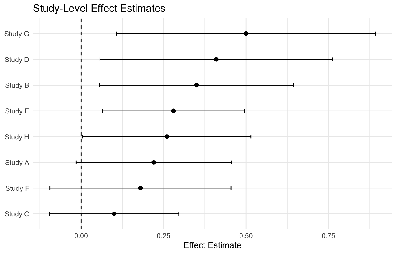
A Small Biostats-Style Example Makes the Workflow Concrete
To illustrate, we will simulate a small set of study-level estimates comparing a treatment versus control effect.
Think of these as coming from a set of clinical or applied biostatistical studies.
# A tibble: 8 × 6
  study      yi   sei     vi    lower upper
  <chr>   <dbl> <dbl>  <dbl>    <dbl> <dbl>
1 Study A  0.22  0.12 0.0144 -0.0152  0.455
2 Study B  0.35  0.15 0.0225  0.056   0.644
3 Study C  0.1   0.1  0.01   -0.096   0.296
4 Study D  0.41  0.18 0.0324  0.0572  0.763
5 Study E  0.28  0.11 0.0121  0.0644  0.496
6 Study F  0.18  0.14 0.0196 -0.0944  0.454
7 Study G  0.5   0.2  0.04    0.108   0.892
8 Study H  0.26  0.13 0.0169  0.00520 0.515
Here:
yi is the study-level effect estimate
sei is the standard error
vi is the variance
This is enough to demonstrate the main meta-analytic ideas.
Forest Plots Are the Signature Visualization of Meta-Analysis
A forest plot is one of the most useful ways to display meta-analytic evidence.
This already gives a useful visual summary of consistency and uncertainty across studies.
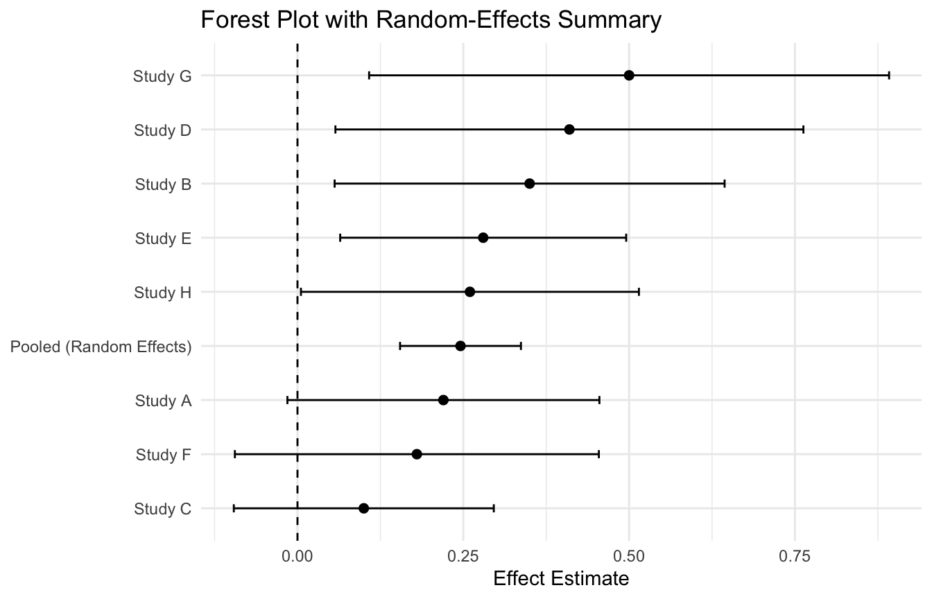
Fixed-Effects Meta-Analysis Assumes One True Common Effect
A fixed-effects meta-analysis assumes that all studies are estimating the same true underlying effect, and that observed differences arise only from sampling error.
Under this model, larger and more precise studies get more weight.
This gives a more recognizable evidence-synthesis visualization.
Fixed and Random Effects Answer Slightly Different Questions
A subtle but important point is that fixed-effects and random-effects models are not only technical alternatives.
They imply different conceptual assumptions.
Fixed effects
Asks, in effect:
what is the common effect if all studies estimate the same truth?
Random effects
Asks:
what is the average effect across a distribution of true study effects?
That difference matters.
In many applied evidence-synthesis settings, especially when studies clearly differ, random effects are often the more realistic default.
But the choice should be justified conceptually, not made automatically.
Meta-Analysis Is About More Than Pooling — It Is Also About Interpretation
A pooled estimate is useful, but it is not the whole story.
Good evidence synthesis also asks:
how consistent are the studies?
are some studies outliers?
is heterogeneity large enough to matter clinically?
are there design differences that explain variation?
is the pooled effect meaningful in the settings where decisions will be made?
This is why meta-analysis is not only a computational exercise. It is also a reasoning framework about how evidence accumulates across contexts.
Bayesian Pooling Makes the Hierarchical Logic Explicit
A Bayesian meta-analysis typically treats study effects as arising from a hierarchical model.
Very loosely:
\[
y_i \sim N(\theta_i, v_i)
\]
and
\[
\theta_i \sim N(\mu, \tau^2)
\]
where:
(y_i) is the observed study effect
(_i) is the true study-specific effect
() is the overall pooled mean effect
(^2) is the between-study heterogeneity
This is conceptually elegant because it makes the partial-pooling structure explicit.
Smaller or noisier studies borrow strength from the overall evidence, while larger studies retain more of their individual influence.
That is one reason Bayesian meta-analysis fits so naturally with modern hierarchical thinking.
Bayesian Meta-Analysis Helps When Uncertainty About Heterogeneity Matters
One advantage of Bayesian pooling is that it treats heterogeneity itself as uncertain rather than plugging in a single estimate (Gelman et al. 2013; Kruschke 2015).
This can be useful when:
the number of studies is small,
heterogeneity is substantial,
or prior knowledge is relevant.
A full Bayesian implementation is more involved than the simple frequentist examples above, but the conceptual takeaway is important:
the pooled effect and the heterogeneity can both be modeled probabilistically.
That often leads to more transparent reasoning about uncertainty.
In AI/ML, Evidence Synthesis Matters When Datasets and Studies Differ
Meta-analytic thinking is increasingly relevant in AI/ML because model training and evidence generation often involve multiple studies, sites, or cohorts.
Examples include:
external validation across hospitals,
federated or multisite evidence synthesis,
combining effect estimates from multiple deployed systems,
or pooling findings from separate model evaluations.
The same core question appears:
how do we combine information without pretending all studies are identical?
That is why meta-analysis is not only for classical clinical trials. It is also useful for evidence-based AI when results must be synthesized across settings.
Heterogeneity in Evidence Synthesis Can Inform Transportability Questions
A pooled estimate can be helpful, but heterogeneity can be even more informative.
If study effects vary meaningfully across settings, that raises important questions:
why do they differ?
which populations resemble the target deployment setting?
is the pooled average the right summary for decision-making?
or do we need subgroup-specific synthesis?
This is where evidence synthesis and transportability start to overlap.
The more heterogeneous the evidence, the more careful the analyst must be about generalization.
Meta-Analysis Can Strengthen Evidence, but It Can Also Pool Bias
A very important caution is that meta-analysis does not automatically create truth.
If the included studies are biased, then meta-analysis may simply synthesize bias more efficiently.
That is why good evidence synthesis depends on:
careful study selection,
study quality assessment,
outcome harmonization,
and thoughtful interpretation.
Pooling weak evidence does not magically produce strong evidence.
This is one reason evidence synthesis should always be paired with methodological judgment.
A Practical R Workflow Often Uses Dedicated Meta-Analysis Packages
For real applied work, analysts usually rely on packages such as:
metafor
meta
bayesmeta
A typical workflow includes:
entering effect estimates and variances,
fitting fixed and random effects models,
generating forest plots,
and exploring heterogeneity or subgroup analyses.
For example, metafor provides a very standard approach.
This is often the most practical route once the conceptual foundations are clear.
A Practical Checklist for Applied Work
Before performing or interpreting a meta-analysis, ask:
What effect measure is being pooled?
Are the studies sufficiently comparable to synthesize meaningfully?
Is a fixed-effects or random-effects model more appropriate conceptually?
How much heterogeneity exists?
Does the pooled estimate hide important differences across settings?
Are study quality and risk of bias being considered?
Would Bayesian pooling better reflect uncertainty in small-study settings?
These questions often matter more than the pooled point estimate itself.
NoteWhere This Shows Up in AI/ML
Federated learning is the ML structural analog of meta-analysis: model parameters or gradients are combined across sites without pooling raw patient data, which is directly relevant to DoD’s distributed health data across MTFs where data governance prohibits central aggregation. Individual MTF sample sizes are often too small to train a reliable trauma mortality model, but the aggregate signal across all facilities is substantial — the same situation that motivates pooling in meta-analysis. High between-site heterogeneity (the I² analog in federated settings) is the signal that a single global model is inappropriate and site-specific or hierarchical models are needed instead. Ignoring heterogeneity and forcing a single federated model across sites with meaningfully different patient populations and injury patterns produces a model that fits no site well.
Closing: Evidence Synthesis Makes Stronger Claims Possible — If Done Thoughtfully
Meta-analysis and evidence synthesis remain essential because important decisions rarely rest on one study alone.
Fixed-effects models provide a common-effect summary when that assumption is plausible. Random-effects models acknowledge that study effects may differ. (I^2) helps describe heterogeneity. Bayesian pooling makes the hierarchical uncertainty structure explicit.
Together, these tools help analysts move from isolated findings toward cumulative evidence.
Meta-analysis matters because stronger evidence often comes not from louder single studies, but from combining multiple studies carefully while respecting where they agree, where they differ, and how uncertain the synthesis still is.
This post is part of the Real-World Evidence Toolkit — a companion reference with fixed and random-effects meta-analysis templates, forest plot code, heterogeneity diagnostics, and Bayesian pooling scaffolds.
DerSimonian, Rebecca, and Nan Laird. 2015. “Meta-Analysis in Clinical Trials Revisited.”Contemporary Clinical Trials 45: 139–45. https://doi.org/10.1016/j.cct.2015.09.002.
Gelman, Andrew, John B. Carlin, Hal S. Stern, David B. Dunson, Aki Vehtari, and Donald B. Rubin. 2013. Bayesian Data Analysis. 3rd ed. Chapman; Hall/CRC.
Higgins, Julian P. T., and Simon G. Thompson. 2002. “Quantifying Heterogeneity in a Meta-Analysis.”Statistics in Medicine 21 (11): 1539–58. https://doi.org/10.1002/sim.1186.
Higgins, Julian P. T., Simon G. Thompson, Jonathan J. Deeks, and Douglas G. Altman. 2003. “Measuring Inconsistency in Meta-Analyses.”BMJ 327 (7414): 557–60. https://doi.org/10.1136/bmj.327.7414.557.
Kruschke, John K. 2015. Doing Bayesian Data Analysis: A Tutorial with R, JAGS, and Stan. 2nd ed. Academic Press.