A treatment effect estimated in one registry, one hospital system, one country, or one trial population may not transport cleanly to a different setting with different:
patient mix,
workflows,
baseline risks,
treatment patterns,
measurement practices,
or site-level resources.
The same is true in AI/ML.
A model can perform well in development and then degrade in deployment because the target population is not the same as the training population.
how transportability differs from internal validity,
why reweighting methods matter,
inverse odds weighting,
and how site-specific effects can be examined in multi-center data.
External validity matters because good answers in one dataset do not automatically become good answers everywhere else.
Internal Validity Is Not the Same as External Validity
A study with strong internal validity gives a credible estimate for the population and setting actually represented in the data.
That is important. But it is not the whole story.
A second question follows immediately:
will this result hold in another population, site, or deployment setting?
That is the question of external validity.
This distinction matters because analysts often stop too early. They focus on whether the estimate is unbiased here, but do not ask whether it applies there.
In real-world evidence and AI deployment, “there” is often the question that matters most.
Generalizability and Transportability Are Closely Related but Not Identical
These terms are often used loosely, but it helps to distinguish them.
Generalizability
Generalizability usually refers to extending results from a study sample to a broader target population that is related to the source population.
Transportability
Transportability often refers to carrying results from one setting into another distinct setting where the target population differs more meaningfully from the source (Stuart et al. 2018; Westreich et al. 2017).
The shared issue is the same:
the source data and the target population are not identical.
That means the analyst must think carefully about whether differences in covariate distribution, treatment practice, or site structure change the result.
External Validity Fails When Effect-Relevant Structure Changes
A result may fail to generalize for many reasons.
For example:
the target population is older or sicker
the treatment is implemented differently
follow-up is shorter
measurement quality differs
healthcare utilization patterns differ
effect modification exists by site or subgroup
The key point is this:
transport fails when the structure that matters for the effect is different across settings.
That is why external validity is not only about sample representativeness in a broad descriptive sense. It is about whether the effect-relevant causal structure remains stable enough across populations.
A Multi-Center RWE Example Makes the Problem Concrete
To illustrate, we will simulate a multi-center real-world evidence setting where:
the source data come mainly from one set of sites,
the target population has a different case mix,
and the treatment effect may vary somewhat by site context.
This is the kind of problem that arises often in comparative effectiveness work and in AI model deployment across institutions.
This setup intentionally creates a source-target population shift.
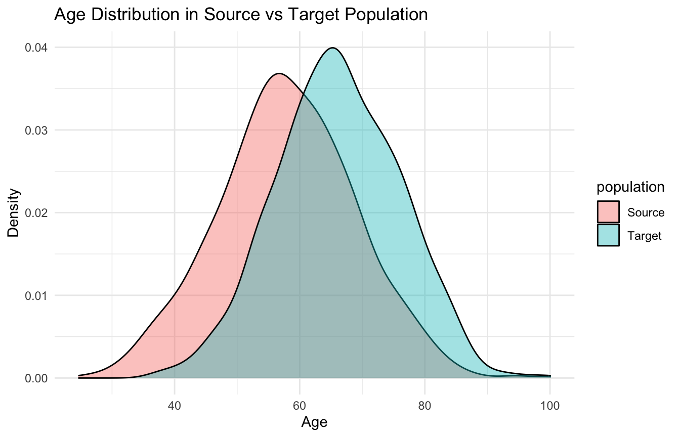
Population Shift Is the First Warning Sign
Before transporting any estimate or model, it is useful to ask a simple question:
how different are the source and target populations?
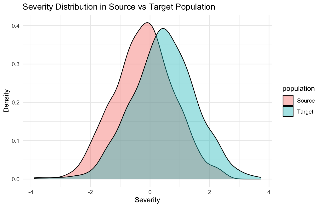
A quick visual can help.
ggplot2::ggplot(transport_df, ggplot2::aes(x = age, fill = population)) + ggplot2::geom_density(alpha =0.4) + ggplot2::labs(title ="Age Distribution in Source vs Target Population",x ="Age",y ="Density" ) + ggplot2::theme_minimal()
We can do the same for severity.
ggplot2::ggplot(transport_df, ggplot2::aes(x = severity, fill = population)) + ggplot2::geom_density(alpha =0.4) + ggplot2::labs(title ="Severity Distribution in Source vs Target Population",x ="Severity",y ="Density" ) + ggplot2::theme_minimal()
These differences do not automatically block transportability, but they signal that naïve reuse of the source estimate may be inappropriate.
External Validity Problems Are Often Covariate Distribution Problems
A key reason transportability fails is that the target population may differ in the distribution of effect modifiers or baseline-risk drivers.
For example:
if older patients respond differently to treatment,
and the target population is older,
then the source average treatment effect may not apply directly.
This means transportability is often tied to the distribution of variables that influence either:
the outcome,
the treatment effect,
or both.
That is why reweighting can be so useful: it tries to make the source sample look more like the target population on relevant observed covariates.
Reweighting Is One of the Main Tools for Transportability
A practical way to transport an estimate is to reweight the source population so that it resembles the target population (Westreich et al. 2017; Stuart et al. 2018).
The basic logic is:
model the probability of belonging to the source versus target population
use those probabilities to create weights
re-estimate the source effect under the weighted source sample
This means the weighted source sample becomes more similar to the target in observed covariates.
The causal idea is that if the key effect-modifying structure is captured in the measured variables, this can improve transportability.
A Simple Sampling Model Helps Build Transport Weights
We begin by modeling whether an observation belongs to the source or target population.
The weighted estimate is not automatically “more true,” but it is more explicitly targeted to the target population under the transport assumptions.
Transportability Depends on Measured Effect Modifiers, Not Just Predictors
A key point is that transportability depends especially on variables that modify the treatment effect or shape baseline risk in ways that matter for the estimand.
Not every covariate difference threatens generalizability equally.
For example:
a variable associated only with source membership but not with the effect may matter less
a variable that strongly modifies treatment response matters much more
This is why transportability is not merely a distribution-matching exercise. It is a causal and scientific reasoning exercise.
The analyst must think carefully about which variables make a result portable or fragile.
Site Effects Are a Practical Threat to External Validity
In multi-center data, one of the most important external-validity questions is:
does the effect differ by site?
This can happen because sites differ in:
case mix,
workflow,
resource availability,
measurement practices,
clinician behavior,
or local treatment implementation.
A model or treatment effect that appears stable overall may hide important site-level heterogeneity.
That is why examining site-specific effects is such an important part of external validity analysis.
Site-Specific Effects Can Be Explored with Interaction Models
A practical first step is to fit a model that allows treatment effects to vary by site.
For a source-only example:
fit_site_int <-glm( outcome ~ treatment * site + age + severity + comorbidity,data = source_analysis_df,family =binomial())summary(fit_site_int)$coefficients[1:9, ]
This kind of model is not the final word on heterogeneity, but it helps answer a key question:
does the treatment effect appear stable across sites, or not?
If site interactions are substantial, simple transport may be much less credible.
Multi-Center Data Are Valuable Because They Reveal Transport Problems Earlier
One major advantage of multi-center data is that they allow external-validity problems to be seen rather than merely hypothesized.
If results vary across centers, that is often a warning that:
the effect is context-sensitive,
the model is site-dependent,
or the deployment setting matters more than the pooled estimate suggests.
This is one reason multi-center evidence is often more informative than a single-site study, even when it is noisier.
It provides a direct opportunity to assess generalizability rather than assuming it.
AI Models Face the Same Problem as Causal Estimates
Everything said so far about transportability of treatment effects also applies to AI models.
A predictive model trained on one population may fail elsewhere because of:
covariate shift,
label shift,
site effects,
measurement differences,
or workflow-driven changes in who gets observed.
This is why external validation is so important in healthcare AI.
A model that performs well internally but poorly across sites is not yet a scalable model.
Generalizability is a deployment question, not just a statistical footnote.
Reweighting Can Also Be Used for Model Performance Transport
In predictive modeling, reweighting can sometimes be used to estimate how a model trained in one dataset might perform in a target population with a different covariate distribution.
The logic is similar:
model source versus target membership,
derive weights,
estimate performance using source observations weighted toward the target population.
This can help answer:
how optimistic is the apparent model performance if the training and deployment populations differ?
That is one of the strongest bridges between causal transportability and AI generalization.
External Validity Still Requires Assumptions
Reweighting and transport methods are powerful, but they are not magic.
They require assumptions such as:
the relevant effect modifiers are measured,
the source and target populations overlap enough,
and the transport model is adequately specified.
If key differences are unmeasured, then even elegant reweighting may fail.
That is why external validity remains partly an empirical problem and partly a scientific judgment problem.
No method can transport an estimate across fundamentally unmeasured context shifts with full confidence.
Trauma Registry Application: External Validity Across Trauma Systems
Trauma registries are often analyzed at the system or network level — but systems differ.
A model trained on a large urban Level I center may not transport to a rural Level III center where:
injury patterns differ (penetrating vs. blunt),
case mix is younger and less comorbid,
resource availability and transfer thresholds differ,
Effect estimates from one trauma system may not generalize to another because effect-modifying variables — ISS distribution, time-to-OR, MTP activation rates — differ across the source and target populations.
Reweighting the source population to resemble the target is one principled approach, but it requires measuring the variables that drive the shift.
For multi-center trauma registries, site effects should be modeled explicitly — not treated as nuisance variation — because they may contain the most clinically actionable information about what works, where, and for whom.
A Practical Checklist for Applied Work
Before claiming that an RWE result or AI model generalizes, ask:
How does the source population differ from the target population?
Are the likely effect modifiers measured?
Is there adequate source–target overlap?
Would transport weights meaningfully improve alignment?
Are site-specific effects present in multi-center data?
Does the result remain stable after reweighting or site-aware modeling?
Am I claiming generalizability beyond what the observed data actually support?
These questions often matter more than the internal model fit.
NoteWhere This Shows Up in AI/ML
The FDA’s framework for AI/ML-based software as a medical device explicitly requires real-world performance monitoring post-deployment — RWE is the ongoing evidence standard for any deployed clinical AI, not just the initial validation. A DoDTR-based trauma mortality model validated on pre-2020 combat data must demonstrate performance stability as injury patterns shift with operational tempo, medical equipment changes, and evolving resuscitation doctrine; a static validation cohort cannot answer this. MHS GENESIS creates the longitudinal data infrastructure to conduct this monitoring, but only if performance metrics — calibration, discrimination, fairness across subgroups — are tracked prospectively rather than retrofitted after a performance failure is noticed clinically. The failure mode is treating deployment as the finish line: models degrade silently when the population they serve drifts from the population on which they were trained.
Closing: External Validity Is Where Evidence Meets the Real World
External validity and generalizability matter because evidence is only useful if it applies where decisions actually need to be made.
A result that is internally valid but not transportable may still mislead in deployment.
Reweighting methods such as inverse odds weighting help align source evidence with target populations. Site-aware analyses help reveal context sensitivity. Multi-center thinking improves realism. And careful external validation keeps analysts from mistaking local success for universal truth.
External validity matters because the real test of evidence is not whether it works where it was created, but whether it still holds when the people, sites, and systems change.
This post is part of the Real-World Evidence Toolkit — a companion reference with transportability reweighting templates, inverse odds weighting code, site-effect diagnostics, and external validity assessment scaffolds.
Cole, Stephen R., and Elizabeth A. Stuart. 2010. “Generalizing Evidence from Randomized Clinical Trials to Target Populations: The ACTG 320 Trial.”American Journal of Epidemiology 172 (1): 107–15. https://doi.org/10.1093/aje/kwq084.
Stuart, Elizabeth A., Brian Ackerman, and Daniel Westreich. 2018. “Generalizability of Randomized Trial Results to Target Populations: Design and Analysis Possibilities.”Research on Social Work Practice 28 (5): 532–37. https://doi.org/10.1177/1049731517720730.
Westreich, Daniel, Jessie K. Edwards, Catherine R. Lesko, Elizabeth Stuart, and Stephen R. Cole. 2017. “Transportability of Trial Results Using Inverse Odds of Sampling Weights.”American Journal of Epidemiology 186 (8): 1010–14. https://doi.org/10.1093/aje/kwx164.