Snapshots in Time: Cross-Sectional Designs for Fast AI Insights
Design of Experiments
An applied introduction to cross-sectional study design, prevalence estimation, association modeling, and the strengths and limits of snapshot data in biostatistics and AI.
Published
February 1, 2026
Modified
June 9, 2026
Executive Summary
Not every study is built to follow people over time.
Sometimes the question is simpler and more immediate:
how common is a condition right now?
how are exposure and outcome related in a population at one point in time?
what baseline structure does the dataset reveal?
what quick insights can be extracted before investing in a more complex design?
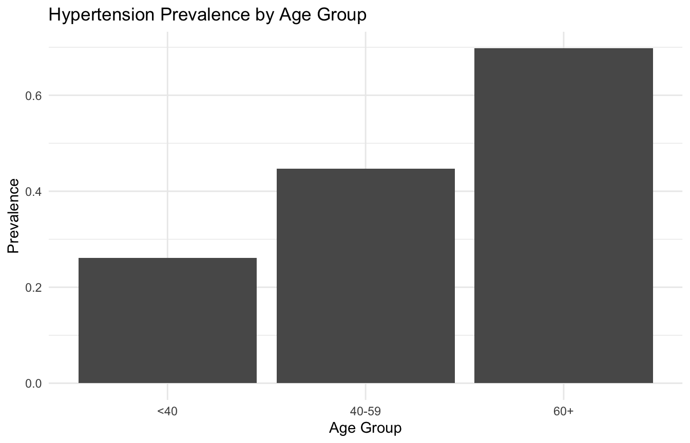
These odds ratios can describe how the odds of prevalent hypertension differ across covariates.
But again, the language matters.
In a cross-sectional study, the result usually supports statements like:
“BMI was associated with higher odds of hypertension”
It is much weaker for claims like:
“higher BMI caused hypertension in this study”
That distinction should stay explicit throughout the post.
10. Cross-Sectional Associations Are Not Automatically Causal
A cross-sectional study can identify associations that are:
clinically interesting
epidemiologically important
operationally useful
or hypothesis-generating
But it usually cannot, on its own, establish:
that exposure preceded outcome
that the association is not reversed
or that the full confounding structure has been addressed
This is why cross-sectional work is often best framed as:
descriptive
associational
exploratory
or prevalence-focused
That is not a weakness of execution. It is a limitation of design.
11. Reverse Causation Is a Constant Risk
One of the most important threats in cross-sectional interpretation is reverse causation(Setia 2016; Rothman et al. 2021).
For example:
low physical activity may be associated with hypertension
but hypertension or related illness may also reduce physical activity
If both are measured at the same time, the analyst cannot easily tell which came first.
This is why temporality is such a central issue.
The same problem appears in many applied settings:
mental health and employment
pain and medication use
symptoms and health-seeking behavior
app engagement and recommendation exposure
Cross-sectional associations can be real and still be directionally ambiguous.
12. Cross-Sectional Design Is Often Useful for Baseline ML Exploration
In AI/ML, cross-sectional data can be valuable for:
clustering
feature screening
descriptive segmentation
baseline risk modeling
and exploratory visualization
These are not necessarily causal tasks.
For example, if the immediate goal is to identify clusters of patients based on a baseline feature snapshot, cross-sectional structure may be enough.
This is one reason cross-sectional designs remain useful in ML. They are often fast ways to understand the shape of the data before more complex longitudinal or causal workflows are attempted.
13. But Cross-Sectional Data Are Weak for Sequential or Intervention Questions
Where cross-sectional design becomes insufficient is in questions involving:
change over time
trajectory prediction
temporal dynamics
treatment sequencing
or intervention effects
Those problems require stronger time structure.
This is why cross-sectional data often serve as a baseline stage in AI/ML, but not as the final design when the scientific goal is forecasting or causal intervention modeling.
That limitation is worth making explicit rather than treating all datasets as interchangeable.
14. Survey Design Quality Matters as Much as the Model
Many cross-sectional studies rely on surveys.
That means the quality of the design depends heavily on:
sampling frame
response rate
measurement quality
weighting
and representativeness
A sophisticated regression model cannot rescue a poorly designed survey.
This is an important lesson in both biostatistics and AI:
model quality does not replace design quality.
In cross-sectional work especially, the design of the sampling and measurement process is often the main determinant of interpretability.
15. Public Survey Data Are Excellent Teaching Tools
Datasets such as NHANES are often excellent for cross-sectional teaching because they offer:
rich measured covariates
health outcomes
strong documentation
and reproducible examples
They are especially good for demonstrating:
prevalence estimation
subgroup visualization
logistic regression associations
and why causal claims should be restrained
That makes them ideal for blog posts or teaching notebooks, even when the final scientific question requires a longitudinal design later.
16. Critiquing Causal Claims Is One of the Best Uses of Cross-Sectional Literacy
A strong learning exercise is not only to analyze a cross-sectional study, but to critique one.
Questions to ask include:
was temporality established?
could reverse causation explain the finding?
was prevalence mistaken for incidence?
did the authors slide from “associated with” into “caused by”?
were key confounders measured?
This critical skill matters a lot because cross-sectional studies are common and often overinterpreted in both scientific and popular reporting.
Being able to recognize what the design can and cannot support is a major sign of statistical maturity.
17. Cross-Sectional Studies Are Often the Right First Study, Not the Final One
One of the most productive ways to view cross-sectional design is as the beginning of an evidence pathway.
A cross-sectional study can help:
describe burden,
identify correlates,
find subgroup patterns,
and motivate stronger follow-up work.
It is often the right design for early insight.
But if the next question becomes:
what predicts future outcomes?
what changes over time?
what is the effect of intervention?
then a stronger temporal design is usually needed.
That is why cross-sectional studies are often most valuable when their limits are recognized clearly.
18. A Practical Checklist for Applied Work
Before designing or interpreting a cross-sectional study, ask:
Is the main goal prevalence estimation, association screening, or something else?
Are exposure and outcome measured at the same time?
Is temporality unknowable from the design?
Could reverse causation explain the association?
Was the sample drawn in a way that supports the target population claim?
Are logistic regression results being interpreted as associations rather than causal effects?
Would a longitudinal design be needed for the real substantive question?
These questions usually matter more than polishing the final regression table.
NoteWhere This Shows Up in AI/ML
Most deployed clinical AI models are structurally cross-sectional — they ingest a snapshot of patient data at a single point in time and return a risk score or classification. This is appropriate for Emergency Severity Index triage scoring or admission-time trauma severity prediction, where the clinical question is genuinely about current state. The failure mode is applying a cross-sectional model to a clinical question that is inherently about trajectory: a patient whose lactate is 4.2 and falling needs a different response than one whose lactate is 4.2 and rising, but a cross-sectional model trained on single observations cannot distinguish them. In DoDTR and MHS GENESIS data, structuring training sets as static snapshots when the outcome is driven by physiologic trajectory produces models that appear well-calibrated in aggregate but systematically misclassify patients undergoing rapid change.
Closing: Cross-Sectional Studies Are Useful When the Question Matches the Snapshot
Cross-sectional designs remain important because they are fast, practical, and often highly informative for the right questions.
They are especially strong for:
prevalence estimation
descriptive epidemiology
and baseline association analysis
But their central limitation is built into the design:
they are weak for temporality and causation.
That is not a flaw. It is a boundary.
Cross-sectional studies matter because a snapshot can reveal a great deal about what is present, but it cannot, by itself, tell the full story of how that pattern emerged or where it is going next.
This post is part of the Real-World Evidence Toolkit — a companion reference with prevalence estimation templates, cross-sectional association reporting scaffolds, and survey-weighted analysis code.
Mann, Christopher J. 2003. “Observational Research Methods. Research Design II: Cohort, Cross Sectional, and Case-Control Studies.”Emergency Medicine Journal 20 (1): 54–60. https://doi.org/10.1136/emj.20.1.54.
Rothman, Kenneth J., Timothy L. Lash, Tyler J. VanderWeele, and Sebastien Haneuse. 2021. Modern Epidemiology. 4th ed. Wolters Kluwer.
Setia, Maninder S. 2016. “Methodology Series Module 3: Cross-Sectional Studies.”Indian Journal of Dermatology 61 (3): 261–64. https://doi.org/10.4103/0019-5154.182410.