Tracking Change: Longitudinal Designs Fueling Predictive AI

Design of Experiments

A practical introduction to longitudinal study design, repeated measures, attrition, mixed-effects thinking, and why trajectories matter in biostatistics and AI.

Published

February 15, 2026

Modified

June 9, 2026

Executive Summary

Some of the most important questions in biostatistics and AI/ML are not about what is true at one moment.

They are about change.

Examples include:

how symptoms evolve after treatment,
how biomarkers drift over repeated visits,
how risk accumulates across time,
how interventions alter trajectories,
and how patient states unfold in sequential data.

These are not snapshot questions. They are longitudinal questions.

A longitudinal study design follows the same individuals or units across multiple time points (Diggle et al. 2002; Fitzmaurice et al. 2011). That repeated-measures structure makes it possible to study:

within-person change,
between-person differences in trajectories,
time-varying predictors,
and attrition or dropout over follow-up.

This matters in both biostatistics and AI/ML.

In biostatistics, longitudinal designs support repeated-measures analysis, mixed-effects models, and intent-to-treat reasoning (Diggle et al. 2002; Fitzmaurice et al. 2011; Bates et al. 2015). In AI/ML, they provide the structure needed for temporal forecasting, disease progression modeling, and sequence-based methods such as recurrent networks or other temporal models.

This post introduces:

what longitudinal designs are,
why they matter,
how repeated measures differ from cross-sectional snapshots,
how attrition complicates interpretation,
and how mixed-effects models and panel-style simulation help make change analyzable.

Longitudinal studies matter because many scientific questions are really questions about trajectories, and trajectories cannot be learned from a single snapshot.

1. Longitudinal Design Begins When Time Becomes Part of the Question

A longitudinal study measures the same unit repeatedly over time.

That unit may be:

a patient,
a clinician,
a hospital,
a household,
a firm,
or a device.

What matters is that the observations are linked across time for the same entity.

This is a fundamentally different design from a cross-sectional study.

A cross-sectional study asks:

what is present now?

A longitudinal study asks:

how does this change across time?

That shift matters because many real-world processes are dynamic rather than static.

2. Repeated Measures Create Both Opportunity and Complexity

Longitudinal data are valuable because they make it possible to study:

baseline differences,
slopes of change,
nonlinear trends,
treatment timing,
relapse and recovery patterns,
and heterogeneity in response.

But repeated measures also create complexity.

Observations from the same person are not independent. That means standard methods that assume independence are often inappropriate.

Longitudinal analysis therefore requires models that respect the dependence structure within subjects.

This is one reason the design and the analysis must be aligned. The data structure itself changes what methods are valid.

3. Longitudinal Designs Are Especially Useful for Trajectory Questions

Many important biomedical and operational questions are really trajectory questions.

For example:

does a treatment reduce symptoms faster over time?
do some patients recover quickly while others decline?
how do ICU severity markers evolve day by day?
do healthcare utilization patterns change before an adverse event?

A longitudinal design is often the natural framework for these questions because it captures both:

between-subject differences
and within-subject change

That combination is one of the biggest strengths of repeated-measures data.

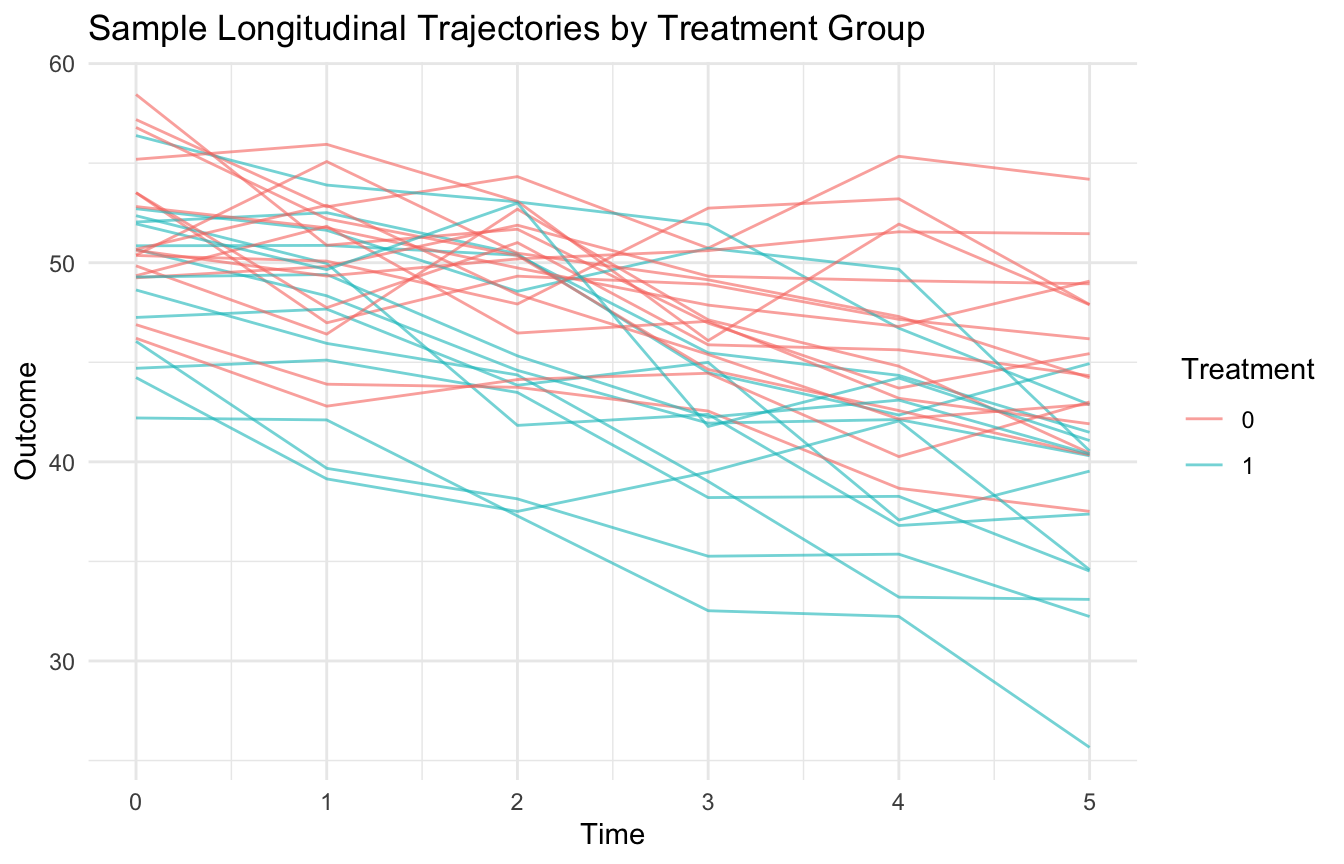
4. A Simple Panel Dataset Makes the Design Concrete

To illustrate, we will simulate a repeated-measures dataset with:

patients observed at multiple follow-up times,
a treatment group,
and an outcome that changes over time.

This is the kind of structure that appears in clinical follow-up and progression studies.

library(dplyr)
library(tibble)
library(ggplot2)

n_subjects <- 180
time_points <- 0:5

long_df <- expand.grid(
  id = 1:n_subjects,
  time = time_points
) |>
  tibble::as_tibble() |>
  dplyr::group_by(id) |>
  dplyr::mutate(
    treatment = rbinom(1, size = 1, prob = 0.5),
    baseline_severity = rnorm(1, mean = 0, sd = 1),
    subject_intercept = rnorm(1, mean = 0, sd = 4),
    subject_slope = rnorm(1, mean = 0, sd = 0.8)
  ) |>
  dplyr::ungroup() |>
  dplyr::mutate(
    outcome = 50 +
      subject_intercept +
      (-1.0 * time) +
      (treatment * -1.5 * time) +
      (-3.0 * baseline_severity) +
      subject_slope * time +
      rnorm(dplyr::n(), mean = 0, sd = 2)
  )

long_df |>
  dplyr::slice_head(n = 10)

# A tibble: 10 × 7
      id  time treatment baseline_severity subject_intercept subject_slope
   <int> <int>     <int>             <dbl>             <dbl>         <dbl>
 1     1     0         1            0.814              2.49        -1.17  
 2     2     0         0           -1.76              -2.60         1.03  
 3     3     0         0            0.489              1.43         0.690 
 4     4     0         0            0.590              4.10        -0.308 
 5     5     0         1           -1.88               0.935       -0.0536
 6     6     0         1           -1.07             -10.3          0.0879
 7     7     0         0            0.766              2.35         0.790 
 8     8     0         1            0.371             -1.56        -1.67  
 9     9     0         0            0.0443             3.24         0.162 
10    10     0         0           -0.428              1.30         0.639 
# ℹ 1 more variable: outcome <dbl>

This gives a patient-by-time dataset where each person contributes repeated outcomes.

5. Plotting Individual Trajectories Is One of the Best First Steps

Before fitting any model, it helps to look at the trajectories.

sample_ids <- long_df |>
  dplyr::distinct(id) |>
  dplyr::slice_sample(n = 30) |>
  dplyr::pull(id)

plot_df <- long_df |>
  dplyr::filter(id %in% sample_ids)

ggplot2::ggplot(plot_df, ggplot2::aes(x = time, y = outcome, group = id, color = factor(treatment))) +
  ggplot2::geom_line(alpha = 0.6) +
  ggplot2::labs(
    title = "Sample Longitudinal Trajectories by Treatment Group",
    x = "Time",
    y = "Outcome",
    color = "Treatment"
  ) +
  ggplot2::theme_minimal()

This type of spaghetti plot makes the repeated-measures structure visible. It shows both:

variation between individuals,
and change within individuals.

That is the essence of longitudinal data.

6. Longitudinal Design Preserves Temporality Better Than Cross-Sectional Design

One of the biggest conceptual advantages of longitudinal design is that it improves temporality.

Repeated measurement makes it easier to ask:

what happened first?
when did the predictor change?
did the outcome worsen before or after intervention?
did decline precede dropout or follow it?

This does not automatically solve all causal problems. But it creates a much stronger temporal structure than a cross-sectional snapshot.

That is why longitudinal designs are often a major step forward when the scientific question involves progression, timing, or response.

7. Attrition Is One of the Central Threats in Longitudinal Studies (Diggle et al. 2002; Fitzmaurice et al. 2011)

Longitudinal designs are powerful, but they are vulnerable to attrition.

Attrition means participants do not all remain under observation for the full follow-up period.

This can happen because of:

dropout,
death,
transfer of care,
loss to follow-up,
nonresponse,
or administrative censoring.

If attrition is related to severity, treatment response, or outcome risk, then the observed longitudinal data may become increasingly selective over time.

That means longitudinal studies often need careful missing-data thinking, not just repeated-measures modeling.

8. Simulating Attrition Helps Show Why It Matters

Let us create a dropout mechanism where patients with worse prior outcomes are more likely to disappear from follow-up.

long_df_attr <- long_df |>
  dplyr::group_by(id) |>
  dplyr::arrange(time, .by_group = TRUE) |>
  dplyr::mutate(
    lag_outcome = dplyr::lag(outcome),
    dropout_prob = dplyr::if_else(
      time == 0,
      0,
      plogis(-6 + 0.08 * lag_outcome)
    ),
    dropout = dplyr::if_else(
      time == 0,
      0L,
      rbinom(dplyr::n(), size = 1, prob = dropout_prob)
    )
  ) |>
  dplyr::mutate(
    ever_drop = cumsum(dropout) > 0,
    outcome_obs = dplyr::if_else(ever_drop & time > 0, NA_real_, outcome)
  ) |>
  dplyr::ungroup()

long_df_attr |>
  dplyr::summarise(
    pct_missing_outcomes = mean(is.na(outcome_obs))
  )

# A tibble: 1 × 1
  pct_missing_outcomes
                 <dbl>
1                0.238

Now the repeated-measures dataset includes informative missingness across time.

9. Longitudinal Studies Often Require Intent-to-Treat Thinking

In trial-like longitudinal settings, intent-to-treat remains an important principle.

The idea is that participants are analyzed according to their originally assigned treatment group, even if:

adherence changes,
switching occurs,
or protocol deviations happen later.

This matters because post-baseline behavior can be related to prognosis. If handled carelessly, excluding or reassigning such participants can reintroduce bias.

Longitudinal studies therefore often need both:

repeated-measures modeling,
and principled rules about how treatment assignment is carried through the analysis.

This is one reason design and analysis remain tightly connected.

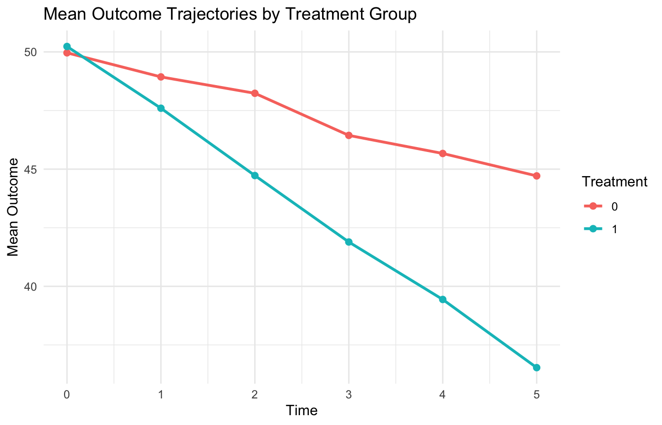
10. Mean Trajectory Plots Are Often a Useful Summary

A useful complement to subject-level plots is a group-level mean trajectory.

mean_traj_df <- long_df |>
  dplyr::group_by(treatment, time) |>
  dplyr::summarise(
    mean_outcome = mean(outcome),
    .groups = "drop"
  )

ggplot2::ggplot(mean_traj_df, ggplot2::aes(x = time, y = mean_outcome, color = factor(treatment))) +
  ggplot2::geom_line(linewidth = 1) +
  ggplot2::geom_point(size = 2) +
  ggplot2::labs(
    title = "Mean Outcome Trajectories by Treatment Group",
    x = "Time",
    y = "Mean Outcome",
    color = "Treatment"
  ) +
  ggplot2::theme_minimal()

This plot is easy to interpret, but it also hides subject-level heterogeneity. That is why it works best alongside individual-level trajectory displays and formal modeling.

11. Repeated Measures Break the Independence Assumption

A major analytical implication of longitudinal design is that repeated observations on the same subject are correlated.

That means methods that assume all rows are independent can underestimate uncertainty and misrepresent structure.

For example:

six observations from one patient are not equivalent to six independent patients.

This is why longitudinal data often call for models such as:

mixed-effects models,
generalized estimating equations,
state-space or time-series methods,
or other subject-aware repeated-measures frameworks.

The dependence structure is not a nuisance detail. It is part of the design.

12. Mixed-Effects Models Are a Natural Starting Point

One of the most common tools for longitudinal analysis is the mixed-effects model.

These models can include:

fixed effects, which describe average population relationships
random effects, which allow subjects to vary in baseline level and sometimes in slope

This is ideal for longitudinal data because different patients often have:

different starting points,
and different rates of change.

A mixed model captures both.

13. A Simple Mixed-Effects Model Shows the Core Longitudinal Logic

Here is a basic linear mixed-effects model with:

time,
treatment,
and a time-by-treatment interaction,
plus a random intercept for subject.

required_pkgs <- c("lme4")
missing_pkgs <- required_pkgs[
  !vapply(required_pkgs, requireNamespace, logical(1), quietly = TRUE)
]

if (length(missing_pkgs) > 0) {
  stop("Missing packages: ", paste(missing_pkgs, collapse = ", "))
}

fit_lmm <- lme4::lmer(
  outcome ~ time * treatment + baseline_severity + (1 | id),
  data = long_df
)

summary(fit_lmm)

The time-by-treatment interaction is especially important because it asks:

does the treatment group change differently over time than the control group?

That is often the main scientific question in a longitudinal trial or repeated follow-up study.

14. Random Slopes Extend the Model to Individual Trajectories

A stronger longitudinal model can also allow each person to have their own slope over time.

fit_lmm_slope <- lme4::lmer(
  outcome ~ time * treatment + baseline_severity + (time | id),
  data = long_df
)

summary(fit_lmm_slope)

This recognizes that not all subjects change in parallel.

Some improve quickly. Some slowly. Some may worsen.

Random slopes are one of the most important ways to represent that heterogeneity explicitly.

15. Longitudinal Data Also Power Sequential AI Models

In AI/ML, longitudinal designs are especially valuable because they provide temporal structure for models that go beyond static prediction.

Examples include:

disease progression forecasting,
treatment response tracking,
wearable signal monitoring,
hospital deterioration prediction,
and sequence-based models.

This is the type of data structure needed for approaches such as:

recurrent neural networks,
LSTMs,
transformers on time-indexed sequences,
and dynamic Bayesian models.

Without repeated measurements, these models lose the very sequence information they are built to exploit.

16. Longitudinal Data Support Dynamic Rather Than Static Prediction

A cross-sectional ML model predicts from a snapshot.

A longitudinal ML model can predict from a path.

That distinction matters because many clinically relevant questions are path-dependent.

For example:

a single lactate value is useful,
but the trend in lactate over repeated time points may be much more informative.

Similarly:

one functional score matters,
but the trajectory of recovery may matter more for prognosis and intervention planning.

Longitudinal study design creates the data structure needed for this kind of dynamic prediction.

17. Repeated Measures Do Not Automatically Solve Causality

It is important not to overclaim.

A longitudinal design is usually stronger than a cross-sectional design for temporality, but it does not automatically solve causal inference.

Problems can still remain, such as:

time-varying confounding,
informative dropout,
measurement error,
treatment switching,
and site-level heterogeneity.

So the main lesson is not that longitudinal studies are automatically causal. It is that they provide a much richer structure for studying change, which can support stronger questions when analyzed carefully.

18. A Practical Checklist for Applied Work

Before designing or analyzing a longitudinal study, ask:

What is the unit being followed?
How many repeated measurements are planned or available?
Is the main question about average trajectory, individual heterogeneity, or intervention effect over time?
How will attrition or dropout be handled?
Is intent-to-treat relevant?
Are repeated measures likely correlated enough to require mixed or marginal models?
Is the scientific question really temporal, or would a simpler cross-sectional design suffice?

These questions usually matter more than jumping straight to a favorite model.

Where This Shows Up in AI/ML

ICU deterioration models, treatment response prediction tools, and readmission risk systems are all longitudinal AI problems where trajectory matters more than any single observation — and LSTM and transformer architectures are specifically designed to exploit that structure. The prerequisite is longitudinal training data with consistent time windows and regular measurement intervals, which MHS GENESIS and DoDTR data require careful preprocessing to provide: irregular observation cadences, missing time points from documentation gaps, and care transitions across facilities all need explicit handling before a model can learn meaningful temporal patterns. When this preprocessing is skipped and repeated-measures data is flattened into wide format for a standard logistic regression, the model discards exactly the information that makes longitudinal design valuable. The design and the architecture must match the clinical question.

Closing: Longitudinal Designs Let Data Tell a Story of Change

Longitudinal studies are powerful because they move analysis beyond static description and into trajectories, timing, and repeated change.

They make it possible to study:

how outcomes evolve,
how treatments alter paths,
how subjects differ in response,
and how predictive systems can learn from sequences instead of snapshots.

But that power comes with demands:

repeated-measures dependence,
attrition,
and more complex modeling choices.

Longitudinal studies matter because many of the most important questions in health and AI are not about what is true at one moment, but about how states evolve, diverge, and respond across time.

📚 Go Deeper: Real-World Evidence Toolkit

This post is part of the Real-World Evidence Toolkit — a companion reference with mixed-effects model templates, trajectory plot scaffolds, attrition documentation standards, and intent-to-treat analysis code.

→ Open the Real-World Evidence Toolkit

Series Callout

Note

This post concludes the series on Design of Experiments for Biostats and AI/ML:

Randomized controlled trials
Observational study designs
Cross-sectional study design
Longitudinal study design
Sample size and power analysis
Stratification and randomization techniques
Blinding and placebo controls
Adaptive study designs
Pragmatic trials
Quasi-experimental designs

Series: Design of Experiments

← Snapshots in Time: Cross-Sectional Designs for Fast AI Insights | Power Up: Avoiding Weak Studies in the AI Era →

References

Bates, Douglas, Martin Mächler, Ben Bolker, and Steve Walker. 2015. “Fitting Linear Mixed-Effects Models Using lme4.” Journal of Statistical Software 67 (1): 1–48. https://doi.org/10.18637/jss.v067.i01.

Diggle, Peter J., Patrick Heagerty, Kung-Yee Liang, and Scott L. Zeger. 2002. Analysis of Longitudinal Data. 2nd ed. Oxford University Press.

Fitzmaurice, Garrett M., Nan M. Laird, and James H. Ware. 2011. Applied Longitudinal Analysis. 2nd ed. Wiley.