A practical guide to sample size and power analysis, including effect size, Type II error, sensitivity analysis, and simulation-based study planning.
Published
March 1, 2026
Modified
June 9, 2026
Executive Summary
A study can be carefully designed, clinically meaningful, and still fail because it is too small (Cohen 1988; Chow et al. 2007).
That is the problem of inadequate power.
Sample size and power analysis matter because they determine whether a study has a reasonable chance to detect an effect that is truly important. In biostatistics, that means reducing the risk of false negatives and unstable estimates. In AI/ML, it means avoiding brittle training, weak validation, subgroup instability, and overfitting driven by too little data.
This post introduces:
what statistical power means,
how to calculate sample size for means and proportions,
how sensitivity analyses help when assumptions are uncertain,
and how simulation makes Type II error visible.
Power analysis matters because a study that cannot reliably detect an important signal is often too weak to answer the question it was built to ask.
1. Sample Size Is a Scientific Design Choice, Not Just a Practical Constraint
Sample size is often discussed as a logistical issue:
how many patients can we recruit?
how much budget do we have?
how long can the study run?
Those are real constraints, but sample size is also a scientific decision.
Too small a study can produce:
low power,
wide confidence intervals,
unstable estimates,
and inconclusive results even when a real effect exists.
Too large a study can also be problematic:
unnecessary cost,
unnecessary participant burden,
and trivial effects appearing statistically compelling.
The right question is not only:
how many observations can we get?
It is:
how many observations do we need to answer the question well?
2. Statistical Power Is the Probability of Detecting a Real Effect
Power is the probability that a study will reject the null hypothesis when a specified true effect exists.
Formally:
\[
\text{Power} = 1 - \beta
\]
where:
\(\beta\) is the probability of a Type II error
a Type II error is failing to detect a real effect
Power depends on:
the true effect size
the sample size
the variability in the data
the significance level
and the chosen analysis
Larger studies usually have more power, but the required size depends heavily on how large the meaningful signal is relative to the noise.
3. Power Calculations Must Be Anchored to a Meaningful Effect Size
A sample size calculation is only as meaningful as the effect it is designed to detect.
That means the analyst must ask:
what difference would actually matter?
For example:
a 5 mmHg blood pressure difference
a 10% event-rate reduction
a 0.05 increase in AUC
a half-day difference in ICU stay
A study powered only for a huge effect may miss smaller but clinically relevant differences. A study powered for an implausibly tiny effect may demand unrealistic sample sizes.
So effect size is not just a mathematical input. It is a scientific choice.
4. A Two-Group Means Comparison Is the Classic Starting Point
A common planning problem is a two-sample comparison of means.
Suppose the outcome is continuous and we want to compare treatment versus control.
The required sample size depends on:
the expected mean difference
the standard deviation
alpha
and the target power
In R, power.t.test() is a straightforward way to do this.
     Two-sample t test power calculation

              n = 99.08057
          delta = 4
             sd = 10
      sig.level = 0.05
          power = 0.8
    alternative = two.sided

NOTE: n is number in *each* group
This estimates the per-group sample size needed to detect a mean difference of 4 units when the standard deviation is 10.
5. Standardized Effect Size Helps Translate Signal Relative to Noise
Sometimes it helps to think in terms of a standardized effect size.
For a two-group mean comparison, Cohen’s \(d\) is:
\[
d = \frac{\mu_1 - \mu_0}{\sigma}
\]
This scales the mean difference by the standard deviation.
     Two-sample comparison of proportions power calculation

              n = 293.1513
             p1 = 0.3
             p2 = 0.2
      sig.level = 0.05
          power = 0.8
    alternative = two.sided

NOTE: n is number in *each* group
This estimates the sample size needed to detect a change from 30% to 20%.
This kind of calculation is common in clinical trials, epidemiology, and ML benchmarking when the endpoint is binary.
7. Alpha and Power Create a Tradeoff
Power planning always involves balancing different risks.
If alpha is made smaller, such as 0.01 instead of 0.05, it becomes harder to declare significance. That generally means a larger sample is needed to achieve the same power.
This means sample size planning is always a compromise among:
Type I error
Type II error
meaningful effect size
and feasibility
There is no universal best answer. The design must reflect the stakes of the problem.
8. Underpowered Studies Do More Than Miss True Effects
The standard lesson is that underpowered studies increase Type II error.
That is true, but incomplete.
Underpowered studies also tend to produce:
unstable estimates
exaggerated significant findings
poor reproducibility
weak subgroup conclusions
That means low power is not only a false-negative problem. It is also a fragility problem.
This matters in AI/ML too, where small datasets can generate noisy models that appear promising but do not generalize.
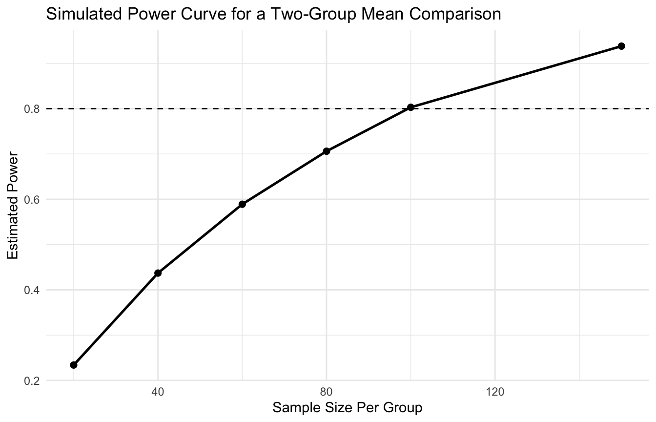
9. Simulation Makes Type II Error Much Easier to Understand
A good way to understand power is to simulate repeated studies under a known true effect.
Suppose the true mean difference is 4 and the standard deviation is 10. We can repeatedly simulate studies and see how often a t-test detects the effect.
This is especially important in longitudinal studies, pragmatic studies, and real-world evidence settings where missingness is rarely trivial.
13. Power Matters in AI/ML Even When It Is Not Called “Power”
In AI/ML, analysts do not always use formal power-analysis language, but the same logic applies.
Too little data can produce:
unstable training
weak generalization
poor subgroup performance
noisy calibration
unreliable validation metrics
This is especially important in:
healthcare ML
rare event modeling
heterogeneous RWE
site-based external validation
So even when the goal is prediction rather than hypothesis testing, the design still needs enough information to support stable learning and credible evaluation.
14. Small Datasets Often Mislead Model Evaluation
When the dataset is too small, model evaluation becomes unstable.
For example:
AUC can vary widely
subgroup metrics become noisy
cross-validation becomes fragile
calibration plots become erratic
That means insufficient sample size can distort not only the model itself, but the analyst’s confidence in the model.
This is one reason data sufficiency matters so much in AI/ML. A weak dataset can make a poor model look promising or a good model look unreliable.
15. Power Analysis Should Match the Primary Goal of the Study
The right sample size depends on the primary goal.
That goal might be:
detecting a treatment effect
comparing event rates
estimating a longitudinal slope
validating a predictive model
or assessing subgroup performance
Different goals imply different formulas and different planning logic.
There is no single universal sample size calculation for all studies.
Power analysis should be built around the primary estimand or primary performance target.
16. Tools Like G*Power Are Useful, but Assumptions Matter More Than Software (Chow et al. 2007)
Software such as G*Power is often helpful for routine design work.
But the most important part of the process is not the software itself. It is the assumptions entered into it.
If the effect size is unrealistic or the variance assumption is poor, the output will still look polished while being scientifically weak.
So software is an implementation aid, not a substitute for design reasoning.
This makes sample size planning not just a statistical issue, but an ethical one.
If the study cannot answer the question reliably, then the design itself may need to be reconsidered.
That is why power analysis is part of responsible study design, not just a reporting requirement.
18. A Practical Checklist for Applied Work
Before finalizing a sample size, ask:
What is the primary estimand or model-performance target?
What effect size would actually matter?
What alpha and power are appropriate for the question?
How uncertain are the assumed variance or event rates?
Has sensitivity analysis been done across plausible assumptions?
Will dropout reduce the analyzable sample?
Is the design large enough for subgroup or validation questions too?
These questions are usually more informative than quoting a single final sample size without context.
NoteWhere This Shows Up in AI/ML
There is no widely adopted standard for sample size requirements in clinical AI model development — a genuine gap that allows underpowered models to reach deployment without scrutiny. Rule-of-thumb guidance exists (10–20 events per predictor variable for logistic regression, 1000+ outcome events for deep learning), but it is rarely formalized in model development reports. Trauma AI models trained on small military treatment facility cohorts produce AUCs with confidence intervals so wide that a reported 0.78 is statistically indistinguishable from 0.62 — making deployment decisions effectively arbitrary. Until the field adopts prospective power analysis as a gate for model development, the DoDTR and GENESIS case volumes available at any single MTF should be treated as a hard constraint on the complexity of models that can be responsibly trained there.
Closing: Power Analysis Helps Ensure the Study Can Actually Answer the Question
Sample size and power analysis are central because they link the scientific question to the amount of information needed to answer it reliably.
That means good planning is not just about formulas. It is about aligning:
effect size
uncertainty
feasibility
and the real study goal
In biostatistics, this reduces weak or inconclusive studies. In AI/ML, it reduces unstable modeling and unreliable validation.
Power analysis matters because collecting data is not the same as collecting enough evidence to support a meaningful conclusion.
This post is part of the Trauma Registry Analytics Toolkit — a companion reference with power calculation templates for registry-based studies, dropout-adjusted sample size scaffolds, and sensitivity analysis grids for effect size assumptions.