library(dplyr)
library(tibble)
library(ggplot2)

n <- 40

simple_assign <- tibble::tibble(
  subject = 1:n,
  arm = sample(c("Control", "Treatment"), size = n, replace = TRUE)
) |>
  dplyr::mutate(
    cum_treat = cumsum(arm == "Treatment"),
    cum_control = cumsum(arm == "Control"),
    imbalance = cum_treat - cum_control,
    design = "Simple randomization"
  )

block_size <- 4
n_blocks <- n / block_size

block_assign <- purrr::map_dfr(
  1:n_blocks,
  function(b) {
    tibble::tibble(
      subject = ((b - 1) * block_size + 1):(b * block_size),
      arm = sample(rep(c("Control", "Treatment"), each = block_size / 2))
    )
  }
) |>
  dplyr::mutate(
    cum_treat = cumsum(arm == "Treatment"),
    cum_control = cumsum(arm == "Control"),
    imbalance = cum_treat - cum_control,
    design = "Blocked randomization"
  )

rand_plot_df <- dplyr::bind_rows(simple_assign, block_assign)Balancing the Scales: Stratification Secrets for Reliable AI
Design of Experiments
A practical introduction to block randomization, stratified randomization, minimization, and post-randomization balance for biostatistics and AI/ML.
Executive Summary
Randomization is one of the strongest protections against bias in study design.
But simple randomization is not always enough.
In smaller studies, or in studies where key baseline covariates strongly influence outcome, chance imbalance can still produce treatment groups that look meaningfully different on variables such as:
- age,
- disease severity,
- site,
- sex,
- or prior treatment exposure.
That is where stratification and randomization techniques become especially useful.
These methods are designed to improve baseline comparability by controlling how treatment assignments are generated. Common approaches include:
- block randomization,
- stratified randomization,
- and minimization.
These design strategies are standard responses to the fact that random assignment protects against systematic allocation bias but does not guarantee exact realized balance in smaller samples. They are discussed in foundational clinical-trial texts and methodological papers on allocation sequence generation and covariate-adaptive assignment (Friedman et al. 2015; Schulz and Grimes 2002; Pocock and Simon 1975).
These ideas matter in both biostatistics and AI/ML.
In trials, they improve group balance and can reduce variance in treatment comparisons. In AI/ML, the same logic appears in stratified sampling and stratified cross-validation, where balanced splits improve fairness and stability, especially in imbalanced real-world data.
This post introduces:
- why randomization alone may not guarantee sufficient balance,
- how block and stratified randomization work,
- what minimization tries to solve,
- how to evaluate post-randomization balance,
- and how these ideas connect to fairer AI evaluation.
Stratification matters because good randomization does not only assign fairly in principle, but also protects against chance imbalances that can weaken interpretation in practice.
1. Simple Randomization Is Powerful, but It Can Still Leave Chance Imbalance
Simple randomization gives each participant an independent probability of assignment to each group.
That is elegant and often sufficient in large trials.
But in smaller or moderate studies, simple randomization can still produce noticeable imbalance in:
- total group sizes,
- baseline severity,
- sex distribution,
- site membership,
- or other important prognostic covariates.
This does not mean simple randomization failed. It means randomization removes systematic bias in expectation, not exact imbalance in every realized sample.
That distinction matters because baseline imbalance can increase variance and complicate interpretation, even when assignment was formally random (Schulz and Grimes 2002; Friedman et al. 2015).
2. Stratification Is a Design Response to Known Prognostic Variables
If certain baseline variables are known in advance to matter strongly, one sensible design response is to stratify on them.
The basic idea is:
- divide participants into strata based on key covariates,
- then randomize within each stratum.
For example, a study might stratify by:
- site,
- sex,
- high versus low severity,
- or age category.
This helps ensure that treatment allocation remains balanced within the clinically important subgroups most likely to distort the comparison if chance imbalance occurs.
That is why stratification is a targeted design choice, not a generic embellishment.
3. Block Randomization Helps Keep Group Sizes Balanced Over Time
A second common technique is block randomization.
The purpose of block randomization is to maintain approximate balance in treatment assignments throughout enrollment rather than only at the end.
For example, in a two-arm trial with 1:1 allocation and block size 4, each block contains:
- two treatment assignments,
- and two control assignments,
but in random order.
This helps prevent long runs of one treatment group during accrual.
That can be especially important when:
- enrollment is slow,
- the study may stop early,
- or site-specific enrollment patterns matter.
4. A Simple Example Shows Why Blocking Helps
Suppose a two-arm study enrolls participants sequentially.
Under simple randomization, the first 20 participants could easily end up with substantial imbalance just by chance.
Under blocked randomization, the imbalance is constrained more tightly across enrollment.
We can compare the two.
Now visualize cumulative imbalance.
ggplot2::ggplot(rand_plot_df, ggplot2::aes(x = subject, y = imbalance, color = design)) +
  ggplot2::geom_line(linewidth = 0.9) +
  ggplot2::geom_hline(yintercept = 0, linetype = 2) +
  ggplot2::labs(
    title = "Cumulative Allocation Imbalance: Simple vs Blocked Randomization",
    x = "Enrollment Order",
    y = "Treatment - Control Count"
  ) +
  ggplot2::theme_minimal()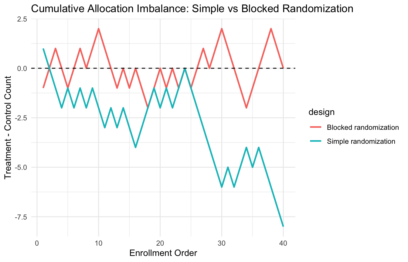
This makes the stabilizing effect of block randomization easy to see.
5. Block Size Affects Predictability and Balance
Block randomization improves balance, but it also introduces a tradeoff.
If the block size is fixed and known, treatment assignment can become somewhat predictable near the end of a block.
That is why many real trials use:
- varying block sizes,
- concealed allocation,
- or both.
The main design lesson is:
- smaller blocks improve short-run balance,
- but may increase predictability,
- while larger blocks reduce predictability but allow more temporary imbalance.
That is why block size should be chosen thoughtfully rather than mechanically.
6. Stratified Randomization Combines Blocking with Clinically Important Covariates
A very common trial design is stratified block randomization.
This means:
- define strata based on one or more important baseline variables
- apply block randomization separately within each stratum
For example, a study might stratify by:
- site,
- baseline severity category,
- and sex,
then randomize in blocks within those subgroups.
This is especially helpful when those variables are strongly related to outcome and imbalance would be concerning.
But there is also a limit: too many strata can make the design sparse and cumbersome.
So stratification should focus on a small number of truly important baseline variables.
7. A Small Stratified Randomization Example Makes the Logic Concrete
Let us simulate participants with:
- site
- severity group
- and treatment assignment via stratified block randomization.
n_subjects <- 120

trial_df <- tibble::tibble(
  id = 1:n_subjects,
  site = sample(c("Site_A", "Site_B", "Site_C"), size = n_subjects, replace = TRUE),
  severity_group = sample(c("Low", "High"), size = n_subjects, replace = TRUE)
) |>
  dplyr::arrange(site, severity_group)

assign_within_stratum <- function(n, block_size = 4) {
  n_full <- n %/% block_size
  rem <- n %% block_size

  assigned <- character(0)

  if (n_full > 0) {
    assigned <- c(
      assigned,
      unlist(
        purrr::map(
          1:n_full,
          ~ sample(rep(c("Control", "Treatment"), each = block_size / 2))
        )
      )
    )
  }

  if (rem > 0) {
    assigned <- c(
      assigned,
      sample(c("Control", "Treatment"), size = rem, replace = TRUE)
    )
  }

  assigned
}

trial_df <- trial_df |>
  dplyr::group_by(site, severity_group) |>
  dplyr::mutate(
    arm = assign_within_stratum(dplyr::n())
  ) |>
  dplyr::ungroup()

trial_df |>
  dplyr::count(site, severity_group, arm)
# A tibble: 12 × 4
site severity_group arm n
<chr> <chr> <chr> <int>
1 Site_A High Control 8
2 Site_A High Treatment 8
3 Site_A Low Control 10
4 Site_A Low Treatment 10
5 Site_B High Control 10
6 Site_B High Treatment 13
7 Site_B Low Control 12
8 Site_B Low Treatment 12
9 Site_C High Control 9
10 Site_C High Treatment 9
11 Site_C Low Control 8
12 Site_C Low Treatment 11This gives a stratified randomization structure across clinically meaningful subgroups.
8. Post-Randomization Balance Should Be Evaluated, Not Assumed
Even when a study uses blocking or stratification, the analyst should still examine baseline balance after randomization.
That means comparing the treatment groups on important covariates.
Common summaries include:
- means and standard deviations for continuous variables
- counts and percentages for categorical variables
- standardized mean differences
- simple balance plots
The point is not to “test the randomization.” It is to understand what the realized sample looks like.
Randomization supports causal validity. Balance diagnostics help describe the realized allocation.
9. Standardized Mean Differences Are a Useful Balance Diagnostic
A common balance measure is the standardized mean difference (SMD).
For a continuous variable, the SMD is:
[ SMD = ]
It expresses group differences in units of pooled variability.
Let us compute balance on age and baseline severity in a simulated randomized sample.
balance_df <- tibble::tibble(
  id = 1:160,
  age = rnorm(160, mean = 59, sd = 11),
  baseline_score = rnorm(160, mean = 0, sd = 1),
  sex = sample(c("Female", "Male"), size = 160, replace = TRUE),
  arm = sample(c("Control", "Treatment"), size = 160, replace = TRUE)
)

smd_cont <- function(x, group) {
  x1 <- x[group == "Treatment"]
  x0 <- x[group == "Control"]
  (mean(x1) - mean(x0)) / sqrt((var(x1) + var(x0)) / 2)
}

balance_tbl <- tibble::tibble(
  variable = c("age", "baseline_score"),
  smd = c(
    smd_cont(balance_df$age, balance_df$arm),
    smd_cont(balance_df$baseline_score, balance_df$arm)
  )
)

balance_tbl
# A tibble: 2 × 2
variable smd
<chr> <dbl>
1 age -0.129
2 baseline_score 0.256This gives a concise numeric summary of post-randomization imbalance.
10. Balance Plots Often Communicate Better Than Tables Alone
A simple dot plot of SMDs can help visualize whether the groups are close on baseline covariates.
ggplot2::ggplot(balance_tbl, ggplot2::aes(x = smd, y = variable)) +
  ggplot2::geom_point(size = 3) +
  ggplot2::geom_vline(xintercept = c(-0.1, 0.1), linetype = 2) +
  ggplot2::labs(
    title = "Post-Randomization Covariate Balance",
    x = "Standardized Mean Difference",
    y = NULL
  ) +
  ggplot2::theme_minimal()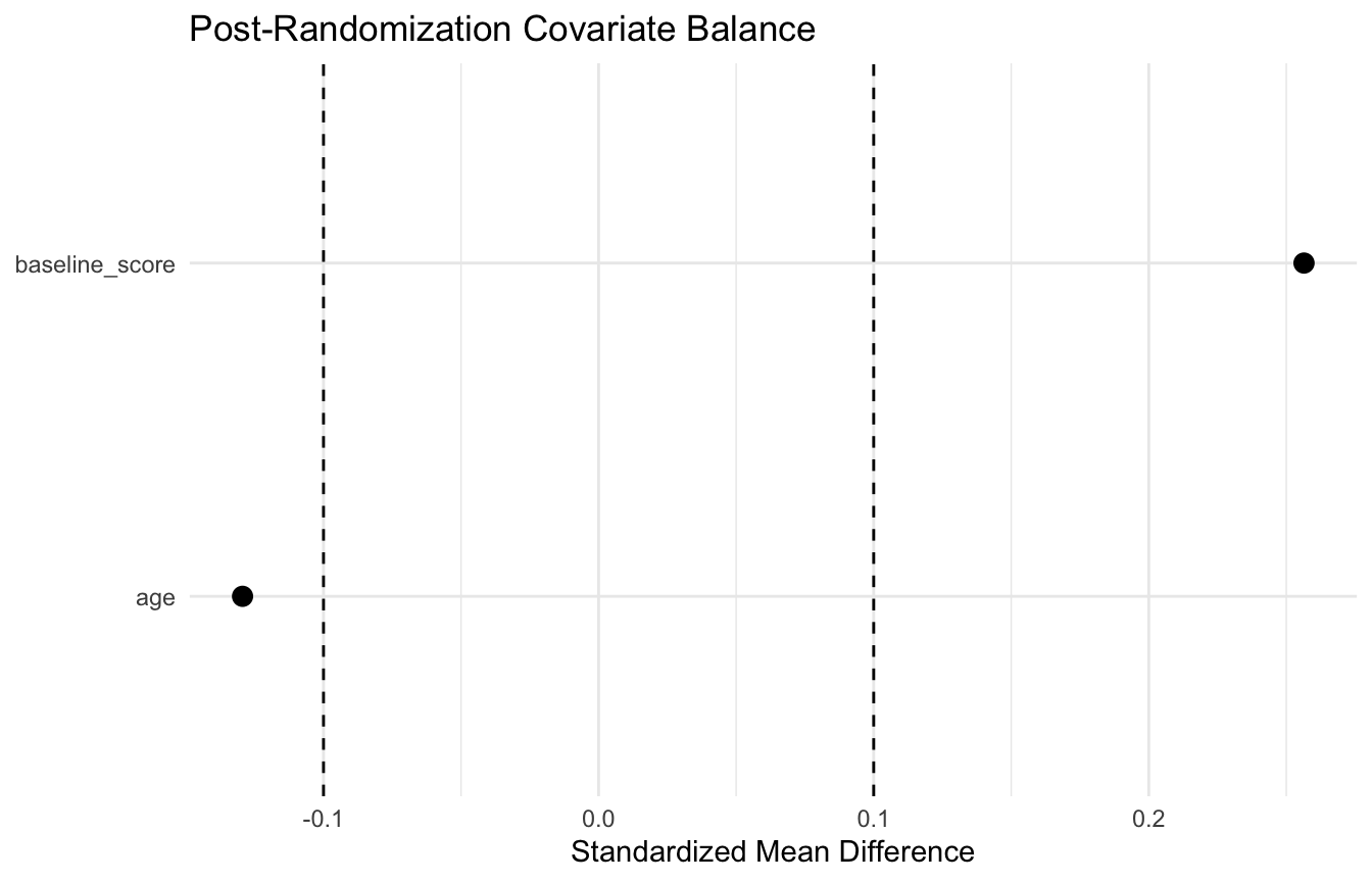
This is often more interpretable than a long baseline table, especially when the number of covariates grows.
11. Minimization Is a More Adaptive Balance Technique (Pocock and Simon 1975; Schulz and Grimes 2002)
When many covariates matter and simple stratification becomes unwieldy, another option is minimization.
Minimization is a dynamic assignment procedure that chooses the treatment allocation for each new participant in a way that reduces overall imbalance across selected covariates.
This is not the same as pure randomization. It is more adaptive.
Usually, minimization includes a random element so that assignments are not fully deterministic.
Minimization is especially useful when:
- sample size is modest,
- multiple important baseline covariates need balancing,
- and traditional stratified blocking would create too many sparse strata.
12. Minimization Solves a Practical Problem: Too Many Strata
If you stratify on:
- site with 5 levels,
- sex with 2 levels,
- severity with 2 levels,
- and disease stage with 3 levels,
you already have:
[ 5 = 60]
possible strata.
That can be cumbersome or sparse in a modest-sized study.
Minimization offers a way to balance across multiple variables without requiring a fully crossed stratum structure.
This is why it is attractive in practice when many prognostic factors matter but the trial is not large enough to support extensive stratification.
13. A Simple Stratified Sampling Script Mirrors the Same Design Logic
The same balancing idea appears outside trials too.
For example, stratified sampling in a dataset ensures that important subgroups are represented proportionally in the sample.
This is conceptually close to stratified randomization.
Here is a simple example of stratified sampling by severity group.
sample_df <- tibble::tibble(
  id = 1:300,
  severity_group = sample(c("Low", "Medium", "High"), size = 300, replace = TRUE, prob = c(0.5, 0.3, 0.2)),
  outcome = rbinom(300, size = 1, prob = 0.25)
)

strat_sample <- sample_df |>
  dplyr::group_by(severity_group) |>
  dplyr::slice_sample(prop = 0.25) |>
  dplyr::ungroup()

sample_df |>
  dplyr::count(severity_group)
# A tibble: 3 × 2
severity_group n
<chr> <int>
1 High 58
2 Low 151
3 Medium 91strat_sample |>
dplyr::count(severity_group)# A tibble: 3 × 2
severity_group n
<chr> <int>
1 High 14
2 Low 37
3 Medium 22This is a simple but useful bridge to ML resampling logic.
14. Stratification Matters in AI/ML Too — Especially in Validation
In AI/ML, the same design logic appears in stratified train/test splits and stratified cross-validation.
Why?
Because when outcomes are imbalanced, random splitting can create folds with very different event proportions.
That can distort performance estimates.
Stratified resampling helps preserve:
- class balance
- subgroup representation
- and more stable evaluation
This is especially important in:
- rare event prediction
- healthcare risk models
- fairness analyses
- and heterogeneous real-world evidence
So the bridge between clinical trial randomization and ML evaluation is not superficial. It is the same balancing idea in a different implementation context.
15. Balance Reduces Variance Even When Bias Is Already Controlled
One subtle but important point is that balance methods are not only about bias.
In a randomized study, bias is already controlled by the randomization mechanism in expectation.
But improved covariate balance can still reduce:
- sampling variance
- instability
- and chance-driven noise in treatment effect estimation
That is why stratification and blocked allocation remain valuable even in settings where simple randomization is already valid.
They do not replace randomization. They refine it.
16. Clinical Trials Often Use Only a Few Stratification Variables for a Reason
A common beginner mistake is to think:
- if some stratification is good, more must be better.
But that is not true.
Too many stratification variables can make implementation difficult and produce sparse subgroups.
In practice, trials often stratify only on a few especially important baseline variables, such as:
- site
- disease severity
- key prognostic marker
This is usually enough to capture the most important sources of imbalance without making the design unwieldy.
That principle is worth stating explicitly.
17. Balance Is a Design Goal, Not a Post Hoc Excuse
One of the strengths of stratification and advanced randomization methods is that they act before the outcome is observed.
That is important.
They do not rescue a poorly balanced study after the fact. They try to prevent avoidable imbalance during assignment itself.
This is one reason design matters so much:
- some problems are much easier to prevent than to fix later with analysis alone.
That is as true in trials as it is in ML data splitting.
18. A Practical Checklist for Applied Work
Before choosing a randomization or stratification scheme, ask:
- Is simple randomization enough for this study size?
- Which baseline covariates are most prognostically important?
- Would block randomization improve allocation balance over time?
- Are there only a few strong variables for stratification, or too many sparse combinations?
- Would minimization be more practical than full stratified blocking?
- How will post-randomization balance be assessed?
- If this were an ML evaluation problem, would stratified splitting be needed for fairness and stability?
These questions usually matter more than choosing the most complicated method available.
NoteWhere This Shows Up in AI/ML
Stratified train/test splitting — ensuring that outcome prevalence, data source, and time period are balanced across training and validation folds — is the direct ML analog of stratified randomization, and skipping it inflates performance estimates in imbalanced clinical datasets. DoDTR trauma mortality models require stratification by theater of operation and injury mechanism to avoid training sets dominated by a single conflict period or casualty pattern; a model trained predominantly on OIF-era blast injuries and validated on the same distribution will report strong performance that evaporates when applied to GWOT-era penetrating trauma or contemporary HADR cases. The failure mode is identical to an unstratified RCT where all high-risk patients end up in one arm: apparent group differences reflect allocation, not treatment. Most published clinical AI papers do not report whether their splits were stratified, which makes their validation results difficult to interpret.
Closing: Stratification Strengthens Randomization by Making Balance More Likely
Stratification and randomization techniques matter because they make a fair comparison more likely in practice, not just in theory.
Simple randomization remains powerful. But block randomization protects group-size balance over enrollment. Stratified randomization protects key prognostic covariates. Minimization helps when many balancing factors matter at once.
And in AI/ML, the same logic appears again in stratified sampling and stratified validation.
Balancing strategies matter because the goal is not only to randomize, but to randomize in a way that protects the comparison from unnecessary instability and chance imbalance.
Tip📚 Go Deeper: Trauma Registry Analytics Toolkit
This post is part of the Trauma Registry Analytics Toolkit — a companion reference with block and stratified randomization templates, balance diagnostic code, and covariate-adaptive allocation scaffolds for multi-site studies.
Series Callout
Note
This post concludes the series on Design of Experiments for Biostats and AI/ML:
- Randomized controlled trials
- Observational study designs
- Cross-sectional study design
- Longitudinal study design
- Sample size and power analysis
- Stratification and randomization techniques
- Blinding and placebo controls
- Adaptive study designs
- Pragmatic trials
- Quasi-experimental designs
References
Friedman, Lawrence M., Curt D. Furberg, David L. DeMets, David M. Reboussin, and Christopher B. Granger. 2015. Fundamentals of Clinical Trials. 5th ed. Springer.
Pocock, Stuart J., and Richard Simon. 1975. “Sequential Treatment Assignment with Balancing for Prognostic Factors in the Controlled Clinical Trial.” Biometrics 31 (1): 103–15. https://doi.org/10.2307/2529712.
Schulz, Kenneth F., and David A. Grimes. 2002. “Generation of Allocation Sequences in Randomised Trials: Chance, Not Choice.” The Lancet 359 (9305): 515–19. https://doi.org/10.1016/S0140-6736(02)07683-3.