How Probability Powers Everyday AI: From Spam Filters to Self-Driving Cars

Applied Statistics
Probability
An applied introduction to probability, contingency tables, Bayes’ theorem, and Monte Carlo simulation for AI and clinical decision-making.
Published

March 15, 2023

Modified

June 9, 2026

Executive Summary

Probability is often taught as a mathematical foundation, but in practice it is also the language of uncertainty in artificial intelligence and machine learning.

This matters in trauma care too.

A trauma team never sees the whole truth at once. Prehospital vitals may be incomplete. Mechanism may be wrong. Hemorrhage may be occult. Laboratory data may lag physiology. Decisions still have to be made.

That is why probability matters: it provides a disciplined way to reason under incomplete information (Kolmogorov 1956; Pearl 1988).

This post introduces:

  • Kolmogorov’s axioms
  • joint, marginal, and conditional probability
  • Bayes’ theorem
  • contingency tables as probability matrices
  • Monte Carlo simulation

AI does not eliminate uncertainty. It formalizes decisions under uncertainty.

Probability Is the Grammar of Uncertainty

In deterministic systems, inputs map cleanly to outputs. In real-world systems, they rarely do.

Data is noisy. Measurements are incomplete. Labels may be uncertain. Signals may conflict.

Probability gives us a framework for answering questions like:

  • How likely is this event?
  • How likely is one event given another?
  • How should new evidence change our beliefs?
  • How much uncertainty remains after prediction?

This is why probability sits underneath so many AI and ML methods (Pearl 1988; Wasserman 2004).

Clinical Translation

For trauma clinicians, probability is not abstract.

  • Marginal probability is the overall mortality in a cohort.
  • Conditional probability is mortality given shock, penetrating injury, or critical transfusion.
  • Joint probability is the probability that two clinical features occur together.
  • Bayesian updating is what happens when suspicion changes after new evidence arrives.
  • Monte Carlo simulation is what we do when repeated scenarios help estimate operational uncertainty.

In other words, probability is one way to formalize what clinicians already do cognitively: update belief as evidence accumulates.

Kolmogorov’s Axioms Define the Rules

All of probability theory begins with three foundational axioms (Kolmogorov 1956).

Let \(A\) be an event in a sample space \(S\).

Axiom 1: Non-negativity

\[ P(A) \geq 0 \]

Axiom 2: Normalization

\[ P(S) = 1 \]

Axiom 3: Additivity

For mutually exclusive events \(A\) and \(B\),

\[ P(A \cup B) = P(A) + P(B) \]

These rules prevent contradiction. A model that assigns incoherent probabilities is not merely poorly calibrated. It is mathematically invalid.

Why These Axioms Matter in AI/ML

Probability axioms underpin practical modeling tasks such as:

  • probabilistic classification,
  • uncertainty quantification,
  • Bayesian updating,
  • ensemble prediction,
  • anomaly detection,
  • and sensor fusion.

If a classifier outputs probabilities that do not cohere, downstream decisions can become misleading or unsafe.

A Simple Toy Example

We will begin with a small email spam example because it is easy to understand and compute. Here, contains_free indicates whether an email contains the word "free" (Yes/No), and spam indicates whether the email is spam (Yes/No).

library(dplyr)
library(tibble)

email_df <- tibble::tibble(
  email_id = 1:20,
  contains_free = c(
    1, 1, 1, 1, 1,
    0, 0, 0, 0, 0,
    1, 1, 0, 0, 1,
    0, 1, 0, 1, 0
  ),
  spam = c(
    1, 1, 1, 0, 1,
    0, 0, 1, 0, 0,
    1, 0, 0, 0, 1,
    0, 1, 0, 1, 0
  )
) |>
  dplyr::mutate(
    contains_free = dplyr::if_else(contains_free == 1, "Yes", "No"),
    spam = dplyr::if_else(spam == 1, "Yes", "No")
  )

email_df
# A tibble: 20 × 3
   email_id contains_free spam 
      <int> <chr>         <chr>
 1        1 Yes           Yes  
 2        2 Yes           Yes  
 3        3 Yes           Yes  
 4        4 Yes           No   
 5        5 Yes           Yes  
 6        6 No            No   
 7        7 No            No   
 8        8 No            Yes  
 9        9 No            No   
10       10 No            No   
11       11 Yes           Yes  
12       12 Yes           No   
13       13 No            No   
14       14 No            No   
15       15 Yes           Yes  
16       16 No            No   
17       17 Yes           Yes  
18       18 No            No   
19       19 Yes           Yes  
20       20 No            No   

Cross Tabulation as a Probability Engine

A two-way contingency table is one of the simplest and most useful probability objects in applied statistics.

It stores the frequency of every combination of two categorical variables. From that single table, we can obtain:

  • joint probabilities,
  • marginal probabilities,
  • conditional probabilities,
  • and tests of whether the two variables appear statistically independent.

This is why contingency tables are so foundational in AI, epidemiology, operations research, and clinical data science.

CrossTable of a Simple 2x2

The gmodels::CrossTable() function prints the table in a SAS PROC FREQ-like format and can optionally report inferential tests and diagnostic summaries.

library(gmodels)

gmodels::CrossTable(
  email_df$contains_free, email_df$spam,
  prop.r = TRUE,        # row proportions
  prop.c = TRUE,        # column proportions
  prop.t = TRUE,        # table proportions (joint probabilities)
  prop.chisq = TRUE,    # chi-square contribution of each cell
  chisq = FALSE,
  fisher = FALSE,
  mcnemar = FALSE,
  resid = FALSE,
  sresid = FALSE,
  asresid = FALSE,
  missing.include = FALSE,
  format = "SAS",
  dnn = c("Contains 'Free'", "Spam")
)

 
   Cell Contents
|-------------------------|
|                       N |
| Chi-square contribution |
|           N / Row Total |
|           N / Col Total |
|         N / Table Total |
|-------------------------|

 
Total Observations in Table:  20 

 
                | Spam 
Contains 'Free' |        No |       Yes | Row Total | 
----------------|-----------|-----------|-----------|
             No |         9 |         1 |        10 | 
                |     2.227 |     2.722 |           | 
                |     0.900 |     0.100 |     0.500 | 
                |     0.818 |     0.111 |           | 
                |     0.450 |     0.050 |           | 
----------------|-----------|-----------|-----------|
            Yes |         2 |         8 |        10 | 
                |     2.227 |     2.722 |           | 
                |     0.200 |     0.800 |     0.500 | 
                |     0.182 |     0.889 |           | 
                |     0.100 |     0.400 |           | 
----------------|-----------|-----------|-----------|
   Column Total |        11 |         9 |        20 | 
                |     0.550 |     0.450 |           | 
----------------|-----------|-----------|-----------|


To save the result as an object:

email_ct <- gmodels::CrossTable(
  email_df$contains_free, email_df$spam,
  prop.r = TRUE,
  prop.c = TRUE,
  prop.t = TRUE,
  prop.chisq = TRUE,
  chisq = FALSE,
  fisher = FALSE,
  mcnemar = FALSE,
  resid = FALSE,
  sresid = FALSE,
  asresid = FALSE,
  missing.include = FALSE,
  format = "SAS",
  dnn = c("Contains 'Free'", "Spam")
)

 
   Cell Contents
|-------------------------|
|                       N |
| Chi-square contribution |
|           N / Row Total |
|           N / Col Total |
|         N / Table Total |
|-------------------------|

 
Total Observations in Table:  20 

 
                | Spam 
Contains 'Free' |        No |       Yes | Row Total | 
----------------|-----------|-----------|-----------|
             No |         9 |         1 |        10 | 
                |     2.227 |     2.722 |           | 
                |     0.900 |     0.100 |     0.500 | 
                |     0.818 |     0.111 |           | 
                |     0.450 |     0.050 |           | 
----------------|-----------|-----------|-----------|
            Yes |         2 |         8 |        10 | 
                |     2.227 |     2.722 |           | 
                |     0.200 |     0.800 |     0.500 | 
                |     0.182 |     0.889 |           | 
                |     0.100 |     0.400 |           | 
----------------|-----------|-----------|-----------|
   Column Total |        11 |         9 |        20 | 
                |     0.550 |     0.450 |           | 
----------------|-----------|-----------|-----------|


What CrossTable() Is Showing

CrossTable() is valuable because it shows multiple views of the same underlying table:

  • email_ct$t is the count table
  • email_ct$prop.tbl is the joint probability table
  • row proportions correspond to probabilities like \(P(\text{Spam} \mid \text{Contains Free})\)
  • column proportions correspond to probabilities like \(P(\text{Contains Free} \mid \text{Spam})\)

In other words, the function is not just printing counts. It is exposing the core probability structure of the data.

Joint Probability

Joint probability describes the probability that two events happen together.

For two categorical variables \(X\) and \(Y\), the joint probability of category \(x_i\) and \(y_j\) is:

\[ P(X = x_i, Y = y_j) \]

In our email example:

\[ P(\text{Contains Free = Yes}, \text{Spam = Yes}) \]

means the probability that an email both contains the word "free" and is spam.

We can calculate the joint probabilities directly:

joint_tbl <- email_df |>
  dplyr::count(contains_free, spam) |>
  dplyr::mutate(prob = n / sum(n))

joint_tbl
# A tibble: 4 × 4
  contains_free spam      n  prob
  <chr>         <chr> <int> <dbl>
1 No            No        9  0.45
2 No            Yes       1  0.05
3 Yes           No        2  0.1 
4 Yes           Yes       8  0.4 

Or obtain them directly from the CrossTable() object:

email_ct$prop.tbl
     y
x       No  Yes
  No  0.45 0.05
  Yes 0.10 0.40

Because the joint probability table represents the full sample space for these two variables, all entries must sum to 1.

sum(email_ct$prop.tbl)
[1] 1

Marginal Probability

Marginal probability is the probability of one variable without conditioning on the other.

For \(X\) and \(Y\):

\[ P(X = x_i) = \sum_j P(X = x_i, Y = y_j) \]

and

\[ P(Y = y_j) = \sum_i P(X = x_i, Y = y_j) \]

These are called marginal probabilities because they appear in the margins of the contingency table.

Marginal Probability for Spam

marginal_spam <- email_df |>
  dplyr::count(spam) |>
  dplyr::mutate(prob = n / sum(n))

marginal_spam
# A tibble: 2 × 3
  spam      n  prob
  <chr> <int> <dbl>
1 No       11  0.55
2 Yes       9  0.45

From the CrossTable() object, the marginal probabilities for spam are the column sums of the joint table:

colSums(email_ct$prop.tbl)
  No  Yes 
0.55 0.45 

Marginal Probability for Contains Free

marginal_free <- email_df |>
  dplyr::count(contains_free) |>
  dplyr::mutate(prob = n / sum(n))

marginal_free
# A tibble: 2 × 3
  contains_free     n  prob
  <chr>         <int> <dbl>
1 No               10   0.5
2 Yes              10   0.5

From the CrossTable() object, the marginal probabilities for contains_free are the row sums:

rowSums(email_ct$prop.tbl)
 No Yes 
0.5 0.5 

Conditional Probability

Conditional probability describes the probability of one event given that another event is known to have occurred.

The general form is:

\[ P(Y = y_j \mid X = x_i) = \frac{P(X = x_i, Y = y_j)}{P(X = x_i)} \]

In our email example, the probability that an email is spam given that it contains the word "free" is:

\[ P(\text{Spam = Yes} \mid \text{Contains Free = Yes}) \]

We can compute it directly:

p_spam_given_free <- email_df |>
  dplyr::filter(contains_free == "Yes") |>
  dplyr::summarise(prob = mean(spam == "Yes")) |>
  dplyr::pull(prob)

p_spam_given_free
[1] 0.8

From CrossTable(), this same idea is represented through the row proportions:

prop.table(email_ct$t, margin = 1)
     y
x      No Yes
  No  0.9 0.1
  Yes 0.2 0.8

The row-normalized table answers questions of the form:

  • among emails with Contains Free = Yes, what proportion are spam?
  • among emails with Contains Free = No, what proportion are spam?

Similarly, column-normalized probabilities can be obtained with:

prop.table(email_ct$t, margin = 2)
     y
x            No       Yes
  No  0.8181818 0.1111111
  Yes 0.1818182 0.8888889

These answer questions of the form:

  • among spam emails, what proportion contain "free"?
  • among non-spam emails, what proportion contain "free"?

Connecting the Table to Matrix Algebra

A useful way to think about a contingency table is as a matrix of joint probabilities.

Let the joint probability matrix be:

\[ \mathbf{P} = \begin{bmatrix} p_{11} & p_{12} \ p_{21} & p_{22} \end{bmatrix} \]

where each element is:

\[ p_{ij} = P(X = x_i, Y = y_j) \]

This matrix view is powerful because:

  • joint probabilities are the matrix entries,
  • marginal probabilities are row or column sums,
  • conditional probabilities are row-normalized or column-normalized versions of the matrix.

If rows represent categories of \(X\) and columns represent categories of \(Y\), then:

\[ P(X = x_i) = \sum_j p_{ij} \]

and

\[ P(Y = y_j) = \sum_i p_{ij} \]

Then conditional probabilities are obtained by dividing each row or column by its corresponding marginal total.

Conceptually, this is exactly what CrossTable() is helping us visualize.

This connection matters because it scales naturally. A simple 2×2 table is easy to draw, but the same mathematical logic extends to:

  • a 3×4 table,
  • a multiway contingency array,
  • or a joint distribution across 6 variables.

Once more variables are introduced, the object is no longer just a matrix. It becomes a higher-dimensional array or tensor. But the same ideas remain:

  • joint distributions store all combinations,
  • marginals collapse across dimensions,
  • conditionals normalize along selected dimensions.

That is one reason probability is so central to modern AI and ML. The mathematical ideas scale from a toy spam filter to much more complex multivariable systems.

Why the CrossTable() Tests Are Useful

Descriptive probabilities tell us what the data look like. Statistical tests help us assess whether the observed association is larger than we would expect from random variation alone.

Chi-Square Test

The chi-square test evaluates whether two categorical variables are statistically independent.

In this example, the null hypothesis is that:

whether an email contains the word "free" is independent of whether it is spam.

If the test is statistically significant, that suggests the variables are associated.

This is usually the default large-sample test for contingency tables.

Fisher’s Exact Test

Fisher’s exact test is also a test of independence, but it is especially useful when sample sizes are small or expected cell counts are sparse.

For small 2×2 tables, Fisher’s test is often more appropriate than the chi-square approximation.

McNemar’s Test

McNemar’s test is different. It is designed for paired 2×2 data, not for ordinary independent observations.

For example, it would be useful if the same emails were classified by two different algorithms, or before and after relabeling. It is generally not the right default for a standard cross-sectional spam table.

Cell Chi-Square Contributions and Residuals

The overall chi-square test may tell us that an association exists, but it does not tell us which cells are driving that association.

That is where these diagnostics help:

  • prop.chisq = TRUE shows how much each cell contributes to the overall chi-square statistic
  • resid = TRUE shows Pearson residuals
  • sresid = TRUE shows standardized residuals
  • asresid = TRUE shows adjusted standardized residuals

These are useful because they identify where observed counts differ most from what we would expect under independence.

For example, if the "Contains Free = Yes" and "Spam = Yes" cell has a large positive residual, that suggests more such emails occur than expected if the variables were unrelated.

A More Inferential Version

If you want to teach or demonstrate both description and inference together, this version is useful:

gmodels::CrossTable(
  email_df$contains_free, email_df$spam,
  prop.r = TRUE,
  prop.c = TRUE,
  prop.t = TRUE,
  prop.chisq = TRUE,
  chisq = TRUE,
  fisher = TRUE,
  mcnemar = FALSE,
  resid = FALSE,
  sresid = TRUE,
  asresid = TRUE,
  missing.include = FALSE,
  format = "SAS",
  dnn = c("Contains 'Free'", "Spam")
)

 
   Cell Contents
|-------------------------|
|                       N |
| Chi-square contribution |
|           N / Row Total |
|           N / Col Total |
|         N / Table Total |
|-------------------------|

 
Total Observations in Table:  20 

 
                | Spam 
Contains 'Free' |        No |       Yes | Row Total | 
----------------|-----------|-----------|-----------|
             No |         9 |         1 |        10 | 
                |     2.227 |     2.722 |           | 
                |     0.900 |     0.100 |     0.500 | 
                |     0.818 |     0.111 |           | 
                |     0.450 |     0.050 |           | 
----------------|-----------|-----------|-----------|
            Yes |         2 |         8 |        10 | 
                |     2.227 |     2.722 |           | 
                |     0.200 |     0.800 |     0.500 | 
                |     0.182 |     0.889 |           | 
                |     0.100 |     0.400 |           | 
----------------|-----------|-----------|-----------|
   Column Total |        11 |         9 |        20 | 
                |     0.550 |     0.450 |           | 
----------------|-----------|-----------|-----------|

 
Statistics for All Table Factors


Pearson's Chi-squared test 
------------------------------------------------------------
Chi^2 =  9.89899     d.f. =  1     p =  0.001653695 

Pearson's Chi-squared test with Yates' continuity correction 
------------------------------------------------------------
Chi^2 =  7.272727     d.f. =  1     p =  0.007000942 

 
Fisher's Exact Test for Count Data
------------------------------------------------------------
Sample estimate odds ratio:  27.32632 

Alternative hypothesis: true odds ratio is not equal to 1
p =  0.005477495 
95% confidence interval:  2.057999 1740.082 

Alternative hypothesis: true odds ratio is less than 1
p =  0.9999405 
95% confidence interval:  0 864.8687 

Alternative hypothesis: true odds ratio is greater than 1
p =  0.002738747 
95% confidence interval:  2.732944 Inf 


Trauma Parallel

The same logic applies to trauma prediction.

Replace "contains_free" with prehospital hypotension and replace "spam" with early critical transfusion or in-hospital mortality.

Then the question becomes:

What is the probability of a poor outcome, given the evidence currently available?

That is the core logic behind risk models, triage tools, and decision-support systems.

And once more than two variables are involved, the same logic extends to richer joint distributions:

  • hypotension,
  • mechanism,
  • injury severity,
  • blood product use,
  • destination role of care,
  • and mortality.

That is already a six-variable probability problem. In practice, modern models estimate or approximate these high-dimensional relationships rather than print a literal six-way table, but the conceptual foundation is the same.
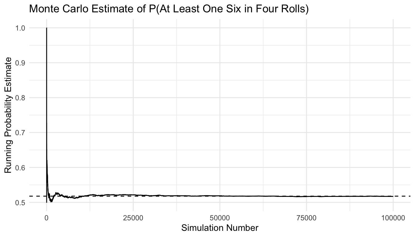
Bayes’ Theorem Updates Belief

Bayes’ theorem formalizes how evidence changes belief (Pearl 1988; Kruschke 2015).

\[ P(A \mid B) = \frac{P(B \mid A)P(A)}{P(B)} \]

p_spam <- email_df |>
  dplyr::summarise(prob = mean(spam == "Yes")) |>
  dplyr::pull(prob)

p_free <- email_df |>
  dplyr::summarise(prob = mean(contains_free == "Yes")) |>
  dplyr::pull(prob)

p_free_given_spam <- email_df |>
  dplyr::filter(spam == "Yes") |>
  dplyr::summarise(prob = mean(contains_free == "Yes")) |>
  dplyr::pull(prob)

p_spam_given_free_bayes <- (p_free_given_spam * p_spam) / p_free

tibble::tibble(
  quantity = c(
    "P(Spam)",
    "P(Contains Free)",
    "P(Contains Free | Spam)",
    "P(Spam | Contains Free)"
  ),
  value = c(
    p_spam,
    p_free,
    p_free_given_spam,
    p_spam_given_free_bayes
  )
)
# A tibble: 4 × 2
  quantity                value
  <chr>                   <dbl>
1 P(Spam)                 0.45 
2 P(Contains Free)        0.5  
3 P(Contains Free | Spam) 0.889
4 P(Spam | Contains Free) 0.8  

Monte Carlo Simulation Makes Probability Operational

Some probabilities are easy to derive analytically. Others are easier to estimate by repeated simulation.

library(ggplot2)

p_exact <- 1 - (5 / 6)^4
n_sims <- 100000

sim_df <- tibble::tibble(
  sim = 1:n_sims,
  die1 = sample(1:6, n_sims, replace = TRUE),
  die2 = sample(1:6, n_sims, replace = TRUE),
  die3 = sample(1:6, n_sims, replace = TRUE),
  die4 = sample(1:6, n_sims, replace = TRUE)
) |>
  dplyr::mutate(
    any_six = die1 == 6 | die2 == 6 | die3 == 6 | die4 == 6,
    running_est = cumsum(any_six) / dplyr::row_number()
  )

p_sim <- sim_df |>
  dplyr::summarise(prob = mean(any_six)) |>
  dplyr::pull(prob)

tibble::tibble(
  method = c("Exact", "Monte Carlo"),
  probability = c(p_exact, p_sim)
)
# A tibble: 2 × 2
  method      probability
  <chr>             <dbl>
1 Exact             0.518
2 Monte Carlo       0.517
ggplot2::ggplot(sim_df, ggplot2::aes(x = sim, y = running_est)) +
  ggplot2::geom_line(linewidth = 0.5) +
  ggplot2::geom_hline(yintercept = p_exact, linetype = 2) +
  ggplot2::labs(
    title = "Monte Carlo Estimate of P(At Least One Six in Four Rolls)",
    x = "Simulation Number",
    y = "Running Probability Estimate"
  ) +
  ggplot2::theme_minimal()

Why This Matters Operationally

Monte Carlo thinking is useful far beyond classroom probability.

It helps analysts explain:

  • uncertainty in outcomes,
  • variability across repeated scenarios,
  • sensitivity to assumptions,
  • and why point estimates can hide operational risk.

That is useful in trauma systems, clinical forecasting, and AI-enabled decision support.

Common Mistakes

Common probability mistakes include:

  • confusing marginal risk with conditional risk,
  • ignoring base rates,
  • overinterpreting rare predictions,
  • and treating model outputs as certainty rather than uncertainty.

These are not just statistical mistakes. They are decision-making mistakes.

NoteWhere This Shows Up in AI/ML

Epic’s sepsis prediction model (Sepsis Watch) outputs a probability score derived from Bayesian updating over sequential vital signs and lab values — the score only makes sense if clinicians understand that it reflects a posterior probability conditioned on the patient’s current trajectory, not a binary alarm. When base rates are ignored — as when the model is deployed in a low-acuity ward where sepsis prevalence is 2% rather than the 20% seen in the ICU training population — the positive predictive value collapses, generating relentless false alarms that erode clinician trust and lead to alert fatigue, the documented failure mode behind several high-profile AI withdrawal decisions in military treatment facilities.

Closing

Probability is central in machine learning. It is the conceptual infrastructure for reasoning under uncertainty (Cover and Thomas 2006; Wasserman 2004).

For clinicians, analysts, and modelers, the core lesson is the same:

Good AI does not remove uncertainty. It represents uncertainty honestly and uses it well.

Series Callout

Note

This post is part of a broader Applied Statistics for AI and Clinical Decision-Making Series:

  • Probability fundamentals for machine learning
  • Random variables and expectation
  • Common probability distributions
  • Central Limit Theorem
  • Law of Large Numbers
  • Sampling methods for Biostats and ML
  • Hypothesis testing in the age of AI
  • Confidence intervals
  • Maximum likelihood estimation
  • Bayesian inference
  • Linear regression
  • Logistic regression
  • Generalized linear models
  • Analysis of variance
  • Principal component analysis
  • Cluster analysis
  • Time series analysis
  • Survival analysis
  • Non-parametric methods
  • Bias-variance tradeoff
  • Regularization
  • Cross-validation
  • Information theory
  • Optimization techniques
  • Linear algebra basics
  • Calculus for ML
  • Monte Carlo methods
  • Dimensionality curse and reduction techniques
  • Model evaluation metrics
  • Ensemble methods

References

Cover, Thomas M., and Joy A. Thomas. 2006. Elements of Information Theory. 2nd ed. Wiley-Interscience.
Kolmogorov, Andrey N. 1956. Foundations of the Theory of Probability. Chelsea Publishing Company.
Kruschke, John K. 2015. Doing Bayesian Data Analysis: A Tutorial with R, JAGS, and Stan. 2nd ed. Academic Press.
Pearl, Judea. 1988. Probabilistic Reasoning in Intelligent Systems: Networks of Plausible Inference. Morgan Kaufmann.
Wasserman, Larry. 2004. All of Statistics: A Concise Course in Statistical Inference. Springer.