Demystifying Random Variables: Why They’re the Secret Sauce in ML Predictions

A practical introduction to random variables, expectation, variance, and expected risk in machine learning and trauma operations.

Executive Summary

Random variables are often introduced early in probability, but their real importance becomes clearer much later.

They allow us to move from talking about uncertain events to talking about uncertain quantities.

Instead of asking only:

• will an event happen or not,
• will a classifier be correct or incorrect,

we begin asking:

• what value might a variable take,
• how large is the expected outcome,
• how variable is that outcome,
• how extreme could the tails be,
• and how should a learning system optimize under uncertainty?

This is where random variables become foundational for machine learning (DeGroot and Schervish 2012; Murphy 2012).

They support:

• probability distributions,
• expectation and variance,
• expected loss,
• optimization under uncertainty,
• simulation-based reasoning.

This also matters in trauma care and operational medicine.

A trauma system does not just face uncertain events. It faces uncertain quantities:

• number of casualties arriving in the next hour,
• units of blood a patient may require,
• time to hemorrhage control,
• ICU days,
• ventilator days,
• mortality risk,
• evacuation delay.

Those are all naturally represented as random variables.

Machine learning models do not optimize single outcomes. They optimize expected behavior across uncertain outcomes.

A Random Variable Turns Uncertainty into Quantity

Probability begins with uncertain events.

Random variables go one step further.

A random variable assigns a numerical value to the outcome of a random process (DeGroot and Schervish 2012; Wasserman 2004).

For example:

• the number showing on a die roll,
• the waiting time until an event occurs,
• the model loss for a randomly sampled observation,
• the return on an asset tomorrow,
• the number of patients arriving in a trauma bay in the next hour.

This shift matters.

It lets us describe not just whether something happens, but how much happens.

That is essential in AI and ML, where models often predict quantities, probabilities, or losses rather than simple yes/no outcomes.

In practice, the random variable is the mathematical bridge between messy reality and a formal model.

Trauma Translation

For trauma clinicians and analysts, random variables are everywhere.

Examples include:

• discrete random variables

  • number of casualties arriving in one hour,
  • number of transfused units in the first 24 hours,
  • number of procedures performed during admission,

• continuous random variables

  • systolic blood pressure,
  • lactate,
  • ICU length of stay,
  • time to definitive hemorrhage control.

This framing matters because different clinical questions imply different kinds of statistical models.

If the variable is a count, a count model may be appropriate. If the variable is continuous, a Gaussian-type model may be a useful starting point. If the variable is binary, the random variable takes values like 0 and 1 and logistic-type models become relevant.

So before fitting any model, one of the first questions should be:

What is the random variable of interest?

Discrete and Continuous Random Variables Represent Different Kinds of Uncertainty

Random variables generally fall into two broad classes.

Discrete Random Variables

A discrete random variable takes values from a countable set.

Examples include:

• number of emails labeled spam,
• number of failed devices in a batch,
• number of casualties arriving in a one-hour period.

A die roll is the classic example.

library(tibble)
library(dplyr)
library(ggplot2)

die_df <- tibble::tibble(
  x = 1:6,
  prob = rep(1 / 6, 6)
)

die_df

# A tibble: 6 × 2
      x  prob
  <int> <dbl>
1     1 0.167
2     2 0.167
3     3 0.167
4     4 0.167
5     5 0.167
6     6 0.167

The table above is a probability mass function for a discrete random variable. It tells us which values are possible and how much probability mass sits on each value.

ggplot2::ggplot(die_df, ggplot2::aes(x = factor(x), y = prob)) +
  ggplot2::geom_col() +
  ggplot2::labs(
    title = "Discrete Random Variable: Fair Die Roll",
    x = "Outcome",
    y = "Probability"
  ) +
  ggplot2::theme_minimal()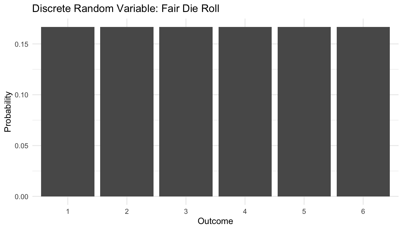

Continuous Random Variables

A continuous random variable can take values across an interval of real numbers.

Examples include:

• blood pressure,
• temperature,
• time to failure,
• model residuals,
• stock returns.

For continuous variables, we talk about density, not point probability.

That distinction matters. For a continuous random variable, the probability of observing any exact single value is effectively zero. Instead, probability is assigned over intervals.

x_grid <- seq(-4, 4, length.out = 500)

norm_df <- tibble::tibble(
  x = x_grid,
  density = dnorm(x_grid, mean = 0, sd = 1)
)

ggplot2::ggplot(norm_df, ggplot2::aes(x = x, y = density)) +
  ggplot2::geom_line(linewidth = 1) +
  ggplot2::labs(
    title = "Continuous Random Variable: Standard Normal Density",
    x = "Value",
    y = "Density"
  ) +
  ggplot2::theme_minimal()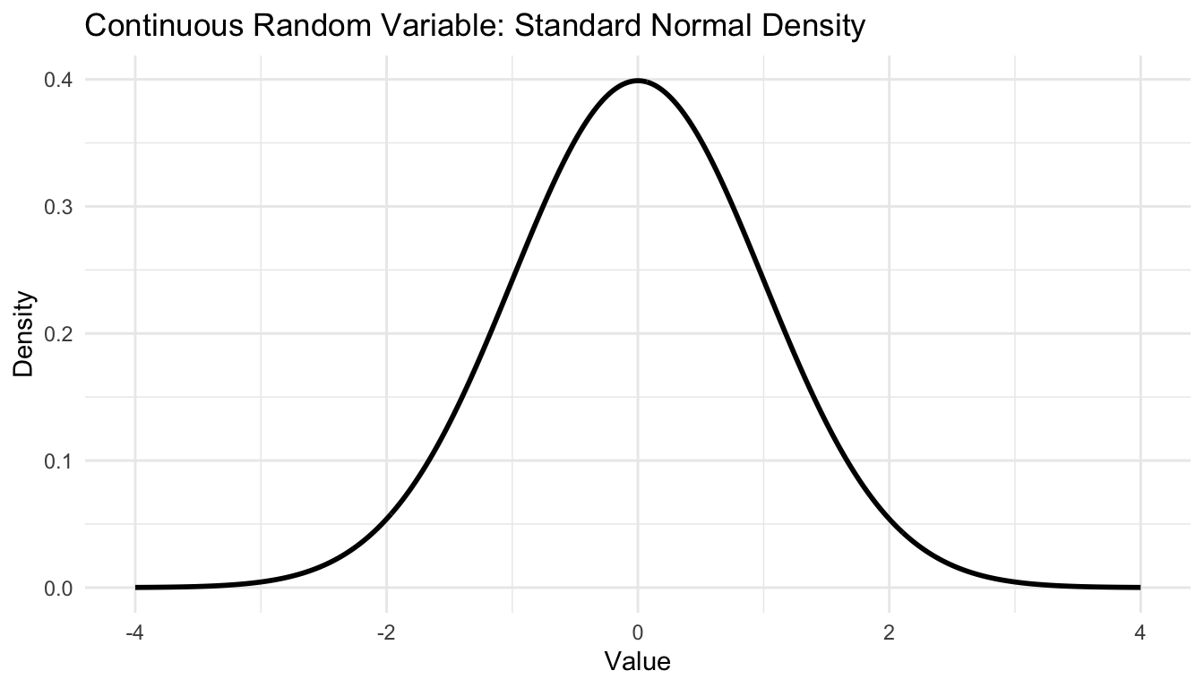

The distinction between discrete and continuous variables is not merely technical.

It affects how we calculate probabilities, expectations, and losses, and it strongly influences the modeling strategy we choose.

The Distribution Tells Us How Uncertainty Is Structured

A random variable is meaningful only together with its distribution.

The distribution tells us:

• which values are possible,
• how likely those values are,
• where the variable tends to concentrate,
• and how much uncertainty surrounds the typical value.

For a discrete random variable, we often use a probability mass function.

For a continuous random variable, we often use a probability density function.

In machine learning, modelers often focus on predictions while forgetting that predictions are embedded in distributions.

But the distribution is the real object of interest whenever uncertainty matters (DeGroot and Schervish 2012; Murphy 2012).

A point prediction without a distributional mindset can hide important facts about:

• volatility,
• rare but consequential outcomes,
• calibration,
• and operational risk.

Expectation Is the Long-Run Average, Not a Guarantee

The expectation or expected value of a random variable is its weighted average value under the distribution (DeGroot and Schervish 2012; Wasserman 2004).

For a discrete random variable:

\[ E[X] = \sum_x x P(X = x) \]

For a continuous random variable:

\[ E[X] = \int x f(x) \, dx \]

Expectation is often interpreted as the long-run average over repeated draws.

For a fair die roll:

expected_die <- sum(die_df$x * die_df$prob)
expected_die

[1] 3.5

The expected value is 3.5.

Of course, no individual roll of a die can produce 3.5.

That is the point.

Expectation is not a prediction of a single outcome. It is a summary of the distribution across repeated uncertainty.

This distinction is crucial in ML.

Expected loss, expected risk, and expected reward are population-level ideas, not guarantees for any single case.

Why Expectation Matters in Trauma and Operations

Expectation is deeply practical.

A planner may ask:

• What is the expected number of casualties arriving in the next hour?
• What is the expected blood utilization for a patient with this injury pattern?
• What is the expected ICU stay for this subgroup?
• What is the expected evacuation delay in a given scenario?

These are expectation questions.

But expected value alone is never the whole story. Two scenarios can have the same expected blood demand but very different tail risk. One may be operationally manageable, while the other may produce occasional catastrophic shortages.

That is why expectation is useful, but insufficient by itself.

Variance Measures How Much Uncertainty Remains Around the Mean

Expectation alone is not enough.

Two random variables can have the same expected value while behaving very differently.

Variance measures the spread around the mean (DeGroot and Schervish 2012):

\[ \mathrm{Var}(X) = E[(X - E[X])^2] \]

For the die example:

variance_die <- sum((die_df$x - expected_die)^2 * die_df$prob)
variance_die

[1] 2.916667

Variance matters because systems do not only care about average behavior.

They also care about stability, volatility, and risk.

A model with low average error but extremely high variability may be unreliable in deployment.

A medical logistics system with manageable average demand but large variance may still fail under surge conditions.

This is why both expectation and variance matter in applied decision-making.

Moments Summarize Important Features of a Distribution

Expectation and variance are examples of more general summary quantities called moments.

Moments help describe features such as:

• center,
• spread,
• asymmetry,
• tail heaviness.

The first moment is the mean.

The second central moment is the variance.

Higher moments often connect to skewness and kurtosis.

In practice, not every applied analyst needs to derive moments by hand, but understanding the idea is useful:

distributions are not just pictures; they can be summarized mathematically in ways that matter for prediction and uncertainty.

This is especially relevant in AI/ML because loss surfaces, residual structures, and predictive uncertainty often depend not just on average behavior, but on broader distributional shape.

Linearity of Expectation Is More Powerful Than It First Appears

One of the most useful properties in probability is linearity of expectation:

\[ E[X + Y] = E[X] + E[Y] \]

More generally,

\[ E[aX + bY] = aE[X] + bE[Y] \]

This holds whether or not the random variables are independent.

That last point is easy to overlook and extremely important.

It means we can compute expected totals without always needing the full joint distribution.

For example, suppose two games each pay random amounts.

game_df <- tibble::tibble(
  outcome = c("Lose", "Win"),
  payoff = c(-1, 3),
  prob = c(0.7, 0.3)
)

expected_game <- sum(game_df$payoff * game_df$prob)
expected_two_games <- expected_game + expected_game

tibble::tibble(
  quantity = c("E[Game 1]", "E[Game 2]", "E[Game 1 + Game 2]"),
  value = c(expected_game, expected_game, expected_two_games)
)

# A tibble: 3 × 2
  quantity           value
  <chr>              <dbl>
1 E[Game 1]            0.2
2 E[Game 2]            0.2
3 E[Game 1 + Game 2]   0.4

This simple idea shows up everywhere:

• expected portfolio return,
• expected model loss over batches,
• expected patient arrivals,
• expected cumulative reward in reinforcement learning.

In trauma systems, it can also apply to expected total blood demand across a set of incoming casualties or expected occupancy burden across a ward or ICU.

Gambling Examples Reveal Why Expected Value Matters

Gambling is often the simplest way to build intuition for expectation.

Suppose a game costs $2 to enter.

You roll one die:

• if you roll a 6, you win $10,
• otherwise, you win $0.

What is the expected net payoff?

gamble_df <- tibble::tibble(
  outcome = c("Roll 6", "Not 6"),
  net_payoff = c(8, -2),
  prob = c(1/6, 5/6)
)

expected_gamble <- sum(gamble_df$net_payoff * gamble_df$prob)
expected_gamble

[1] -0.3333333

Even when a game has a positive expected value, it may still involve substantial uncertainty.

That is why expectation is necessary but not sufficient.

In ML, this parallels the difference between:

• low expected loss,
• and stable, reliable performance.

Stock Simulations Provide Another Useful Intuition

Financial returns are a familiar example of uncertain quantities.

Suppose a stock has daily returns modeled as approximately normal with:

• mean return = 0.0005
• standard deviation = 0.02

We can simulate many possible one-day returns.

sim_returns <- tibble::tibble(
  return = rnorm(10000, mean = 0.0005, sd = 0.02)
)

sim_returns |>
  dplyr::summarise(
    mean_return = mean(return),
    var_return = var(return),
    sd_return = sd(return)
  )

# A tibble: 1 × 3
  mean_return var_return sd_return
        <dbl>      <dbl>     <dbl>
1    0.000737   0.000400    0.0200

ggplot2::ggplot(sim_returns, ggplot2::aes(x = return)) +
  ggplot2::geom_histogram(bins = 50) +
  ggplot2::labs(
    title = "Simulated Daily Stock Returns",
    x = "Return",
    y = "Count"
  ) +
  ggplot2::theme_minimal()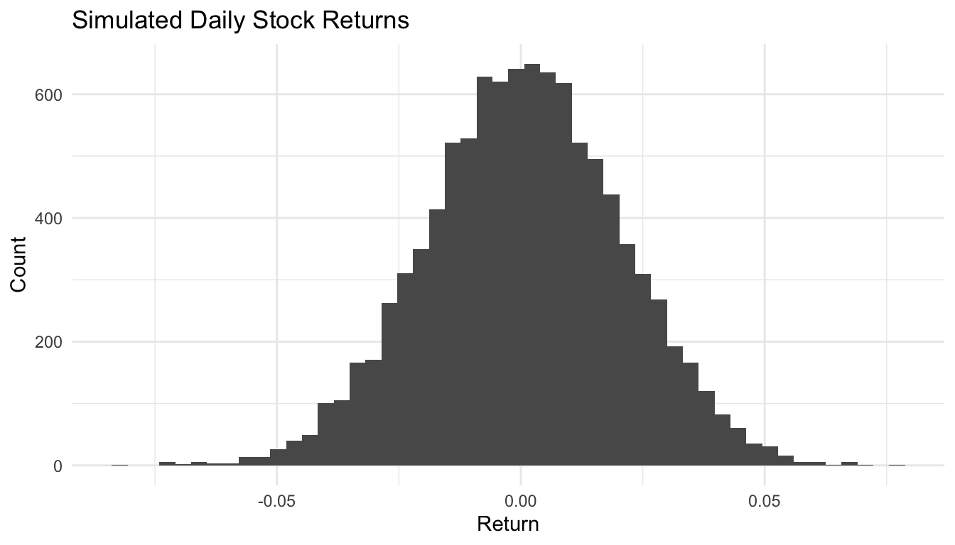

This example is useful because it illustrates several ideas at once:

• a random variable can represent a real-valued uncertain quantity,
• expectation summarizes average behavior,
• variance captures volatility,
• simulation makes the uncertainty visible.

A Trauma Example in R: Arrival Counts as a Random Variable

To connect this more directly to trauma operations, suppose the number of casualties arriving in one hour is modeled as a count random variable.

A common starting point for counts is the Poisson distribution.

Let:

\[ X = \text{number of casualty arrivals in one hour} \]

and suppose:

\[ X \sim \text{Poisson}(\lambda = 3) \]

Then the expected number of arrivals in an hour is 3.

arrival_df <- tibble::tibble(
  x = 0:10,
  prob = dpois(0:10, lambda = 3)
)

arrival_df

# A tibble: 11 × 2
       x     prob
   <int>    <dbl>
 1     0 0.0498  
 2     1 0.149   
 3     2 0.224   
 4     3 0.224   
 5     4 0.168   
 6     5 0.101   
 7     6 0.0504  
 8     7 0.0216  
 9     8 0.00810 
10     9 0.00270 
11    10 0.000810

ggplot2::ggplot(arrival_df, ggplot2::aes(x = factor(x), y = prob)) +
  ggplot2::geom_col() +
  ggplot2::labs(
    title = "Trauma Example: Hourly Casualty Arrivals",
    x = "Number of Arrivals",
    y = "Probability"
  ) +
  ggplot2::theme_minimal()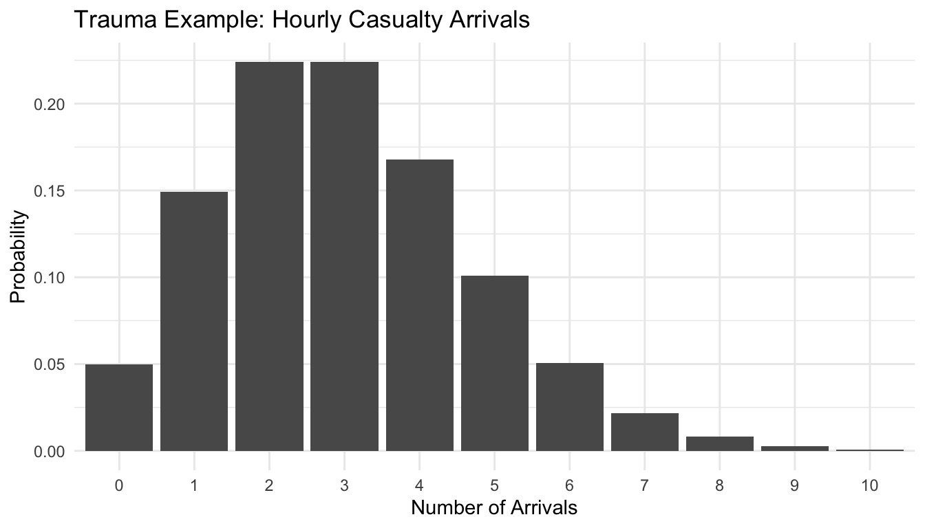

Now compute the expected value and variance directly from the distribution.

expected_arrivals <- sum(arrival_df$x * arrival_df$prob)
variance_arrivals <- sum((arrival_df$x - expected_arrivals)^2 * arrival_df$prob)

tibble::tibble(
  quantity = c("Expected arrivals", "Variance"),
  value = c(expected_arrivals, variance_arrivals)
)

# A tibble: 2 × 2
  quantity          value
  <chr>             <dbl>
1 Expected arrivals  3.00
2 Variance           2.98

This kind of thinking can support:

• staffing decisions,
• surge planning,
• blood product preparation,
• transport readiness,
• and simulation-based logistics.

Expected Risk Minimization Sits at the Heart of Machine Learning

One of the most important reasons random variables matter in ML is that learning is often framed as expected risk minimization (Murphy 2012).

Very loosely, the goal is to find a model \(f\) that minimizes the expected loss:

\[ R(f) = E[L(Y, f(X))] \]

where:

• \(X\) is the input,
• \(Y\) is the target,
• \(L\) is the loss function.

This equation is central.

It says the model is not judged on a single observation, but on its average loss across the distribution of possible data.

That is expectation doing the work.

In practice, empirical risk minimization approximates this expectation with sample averages.

But conceptually, the target is still expected loss under uncertainty.

This is one reason random variables are not optional background theory. They are embedded directly in how learning objectives are defined.

Gradient Descent Also Depends on Expectations

Even optimization methods like gradient descent are easier to understand once expectation enters the picture.

When training models, we often estimate gradients using samples or mini-batches.

These sample-based gradients can be viewed as noisy estimates of an underlying population gradient.

In other words, optimization often proceeds by using realized samples to approximate expected quantities.

This is one reason probabilistic thinking matters even in systems that are not explicitly Bayesian.

Randomness is not peripheral. It is built into the data-generating process, the objective function, and often the optimization itself (Murphy 2012).

Simulation Helps Make Random Variables Concrete

One of the best ways to teach random variables is to simulate repeated draws and watch the empirical behavior develop.

For example, here we repeatedly roll a die and track the running average.

n_sims <- 5000

sim_die <- tibble::tibble(
  draw = 1:n_sims,
  value = sample(1:6, n_sims, replace = TRUE)
) |>
  dplyr::mutate(
    running_mean = cumsum(value) / dplyr::row_number()
  )

head(sim_die)

# A tibble: 6 × 3
   draw value running_mean
  <int> <int>        <dbl>
1     1     2         2   
2     2     1         1.5 
3     3     5         2.67
4     4     5         3.25
5     5     4         3.4 
6     6     3         3.33

ggplot2::ggplot(sim_die, ggplot2::aes(x = draw, y = running_mean)) +
  ggplot2::geom_line(linewidth = 0.5) +
  ggplot2::geom_hline(yintercept = expected_die, linetype = 2) +
  ggplot2::labs(
    title = "Running Average of Repeated Die Rolls",
    x = "Simulation Number",
    y = "Running Mean"
  ) +
  ggplot2::theme_minimal()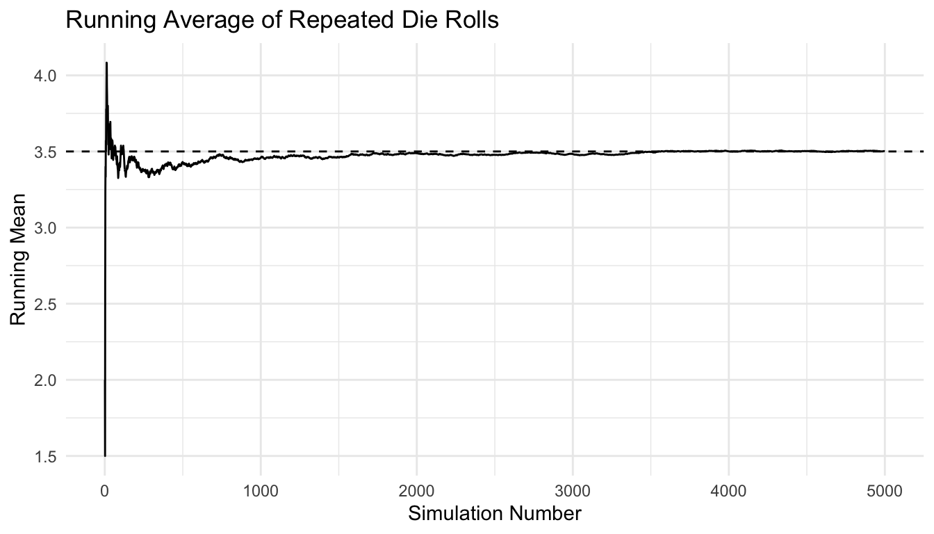

This makes the abstract idea of expectation more concrete. The expected value is not the outcome of one draw. It is the value toward which the long-run average tends to stabilize.

That idea sits behind many simulation methods in AI, ML, and operations research.

Visualizing How Parameters Change Distributions

One of the best ways to teach random variables is to visualize how distributions change as parameters change.

For example, here is a simple illustration using normal densities with different means and standard deviations.

param_df <- tibble::tribble(
  ~mean, ~sd, ~label,
   0,     1,  "mean = 0, sd = 1",
   1,     1,  "mean = 1, sd = 1",
   0,     2,  "mean = 0, sd = 2"
)

plot_df <- param_df |>
  dplyr::rowwise() |>
  dplyr::do(
    tibble::tibble(
      x = seq(-6, 6, length.out = 400),
      density = dnorm(seq(-6, 6, length.out = 400), mean = .$mean, sd = .$sd),
      label = .$label
    )
  ) |>
  dplyr::ungroup()

ggplot2::ggplot(plot_df, ggplot2::aes(x = x, y = density)) +
  ggplot2::geom_line(linewidth = 1) +
  ggplot2::facet_wrap(~ label, scales = "free_y") +
  ggplot2::labs(
    title = "How Distribution Parameters Change a Continuous Random Variable",
    x = "Value",
    y = "Density"
  ) +
  ggplot2::theme_minimal()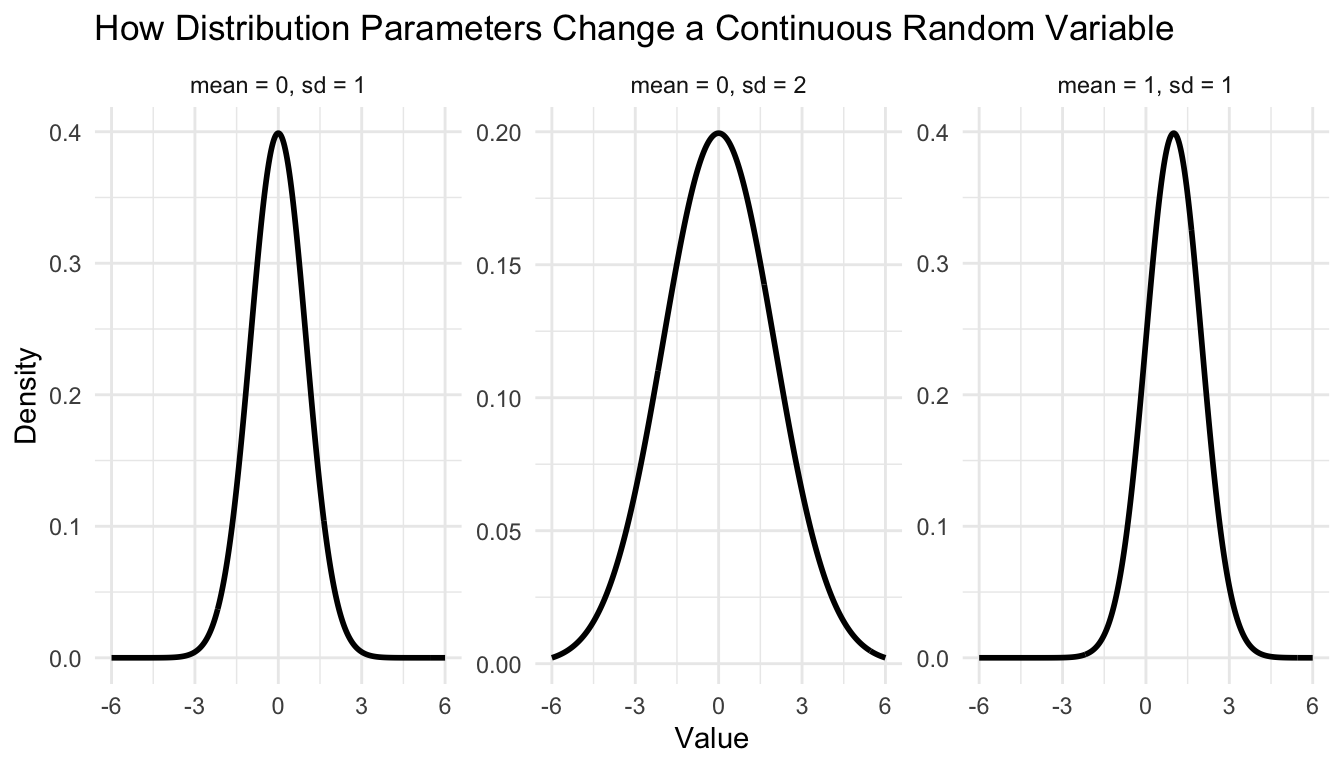

In a fuller Quarto website workflow, you could make these truly interactive with plotly, html widgets, or Shiny components.

But even static visuals go a long way toward making the ideas less abstract.

Random Variables Are the Bridge Between Data and Decisions

Random variables are not just a technical definition.

They are the bridge between:

• uncertain reality,
• mathematical representation,
• model-based prediction,
• and real decisions.

Without random variables, we cannot define:

• expected loss,
• uncertainty intervals,
• probabilistic forecasts,
• risk-sensitive strategies,
• or the distributional assumptions behind most statistical learning methods.

They are not background machinery. They are part of the conceptual engine.

A Practical Checklist for Applied Work

Before using a model or stochastic system, ask:

• What is the random variable of interest?
• Is it discrete or continuous?
• What distribution is being assumed or estimated?
• What is the expected value?
• How variable is the outcome?
• Is the average behavior enough, or do tails and volatility matter?
• Is the objective function minimizing observed error or expected risk?

These questions sharpen both modeling and interpretation.

NoteWhere This Shows Up in AI/ML

Every output of a clinical prediction model — a mortality probability, a readmission risk score, a triage acuity classification — is a realization of a random variable with a full distribution, not a fixed number; the model’s softmax output represents E[Y | X], the expected value of the outcome given features, and treating it as a deterministic answer rather than a distribution summary discards the variance information that determines whether any individual prediction should be acted on. In trauma triage systems deployed at Role 2 and Role 3 facilities, reporting a point estimate of 0.73 mortality risk without communicating prediction variance means two patients with the same score but very different uncertainty levels receive identical resource allocation — a clinically consequential error that the random-variable framing would prevent.

Closing: Expectation Is About More Than Averaging

Random variables allow us to treat uncertainty as something measurable.

Expectation gives us a way to summarize long-run average behavior. Variance tells us how much uncertainty remains. Moments reveal additional structure. Linearity of expectation makes complex systems tractable.

In machine learning, these are not ornamental ideas.

They explain why loss functions work, why optimization behaves the way it does, and why predictions must be understood as summaries of uncertainty rather than deterministic truths.

In trauma analytics, they help frame operational questions rigorously:

• expected arrivals,
• expected blood demand,
• expected ICU burden,
• expected evacuation delay,
• and the uncertainty around all of them.

Random variables are not just mathematical abstractions. They are how models translate uncertainty into prediction, risk, and action.

Tip📚 Go Deeper: Prediction Modeling Toolkit

This post is part of the Prediction Modeling Toolkit — a companion reference with feature engineering templates, distribution diagnostics, and simulation-based modeling scaffolds.

→ Open the Prediction Modeling Toolkit

Series Callout

Note

This post is part of a broader Applied Statistics for AI and Clinical Decision-Making Series:

• Probability fundamentals for machine learning
• Random variables and expectation
• Common probability distributions
• Central Limit Theorem
• Law of Large Numbers
• Sampling methods for Biostats and ML
• Hypothesis testing in the age of AI
• Confidence intervals
• Maximum likelihood estimation
• Bayesian inference
• Linear regression
• Logistic regression
• Generalized linear models
• Analysis of variance
• Principal component analysis
• Cluster analysis
• Time series analysis
• Survival analysis
• Non-parametric methods
• Bias-variance tradeoff
• Regularization
• Cross-validation
• Information theory
• Optimization techniques
• Linear algebra basics
• Calculus for ML
• Monte Carlo methods
• Dimensionality curse and reduction techniques
• Model evaluation metrics
• Ensemble methods

Series: Applied Statistics for AI & Clinical Decision-Making

← How Probability Powers Everyday AI: From Spam Filters to Self-Driving Cars  |  Top Probability Distributions Every Data Scientist Needs: Visual Guides and ML Applications →

References

DeGroot, Morris H., and Mark J. Schervish. 2012. Probability and Statistics. 4th ed. Pearson.

Murphy, Kevin P. 2012. Machine Learning: A Probabilistic Perspective. MIT Press.

Wasserman, Larry. 2004. All of Statistics: A Concise Course in Statistical Inference. Springer.