This idea is one of the most important concepts in both statistics and machine learning because it explains why better fit on training data does not always lead to better prediction on new data (Hastie et al. 2009; James et al. 2021).
At the center of the tradeoff is a simple truth:
a model can be wrong because it is too rigid, or wrong because it is too unstable.
This post introduces:
bias and variance intuitively,
mean squared error decomposition,
simulation with polynomial regression,
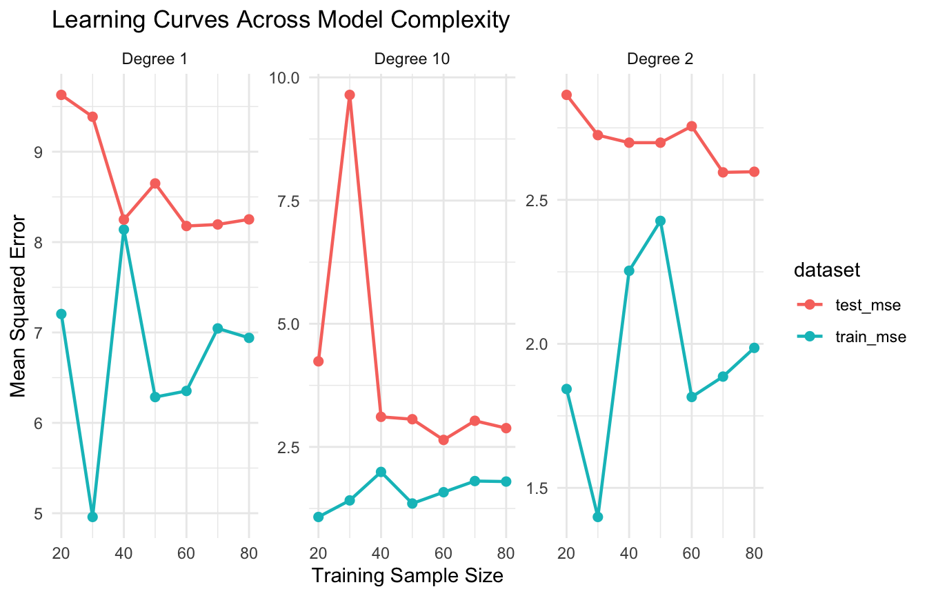
learning curves,
and why this tradeoff matters for regularization, ensembles, and model selection.
The best predictive model is usually not the one that fits hardest, but the one that balances systematic error against instability.
The Bias-Variance Tradeoff Explains Why Prediction Is Hard
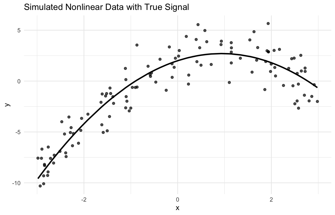
A model can fail in two broad ways.
It can be too simple to represent the true signal. That creates bias.
Or it can be too sensitive to sample-specific noise. That creates variance.
These two problems usually pull in opposite directions.
As flexibility increases:
bias often decreases,
but variance often increases.
As flexibility decreases:
variance often decreases,
but bias often increases.
This is why predictive modeling is rarely about maximizing fit alone. It is about finding an appropriate level of complexity.
Bias and Variance Reflect Different Kinds of Error
Bias
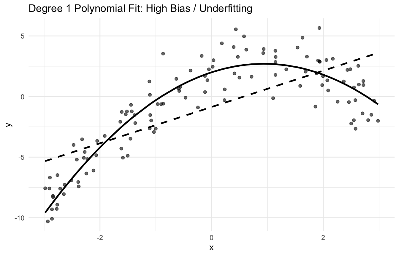
Bias refers to systematic error.
A high-bias model tends to miss important structure in the data repeatedly. Even across many samples, it keeps making errors in the same general direction.
This is often associated with underfitting.
Variance
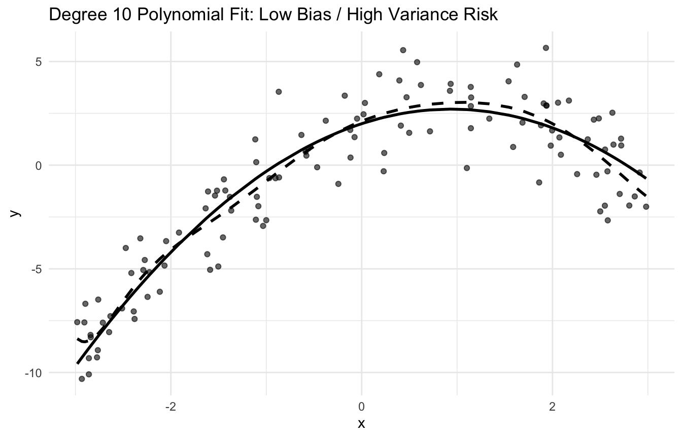
Variance refers to instability.
A high-variance model may fit one sample very differently from another. Its predictions are highly sensitive to the specific data observed.
This is often associated with overfitting.
These are different failure modes. A model can be stable but wrong, or flexible but erratic.
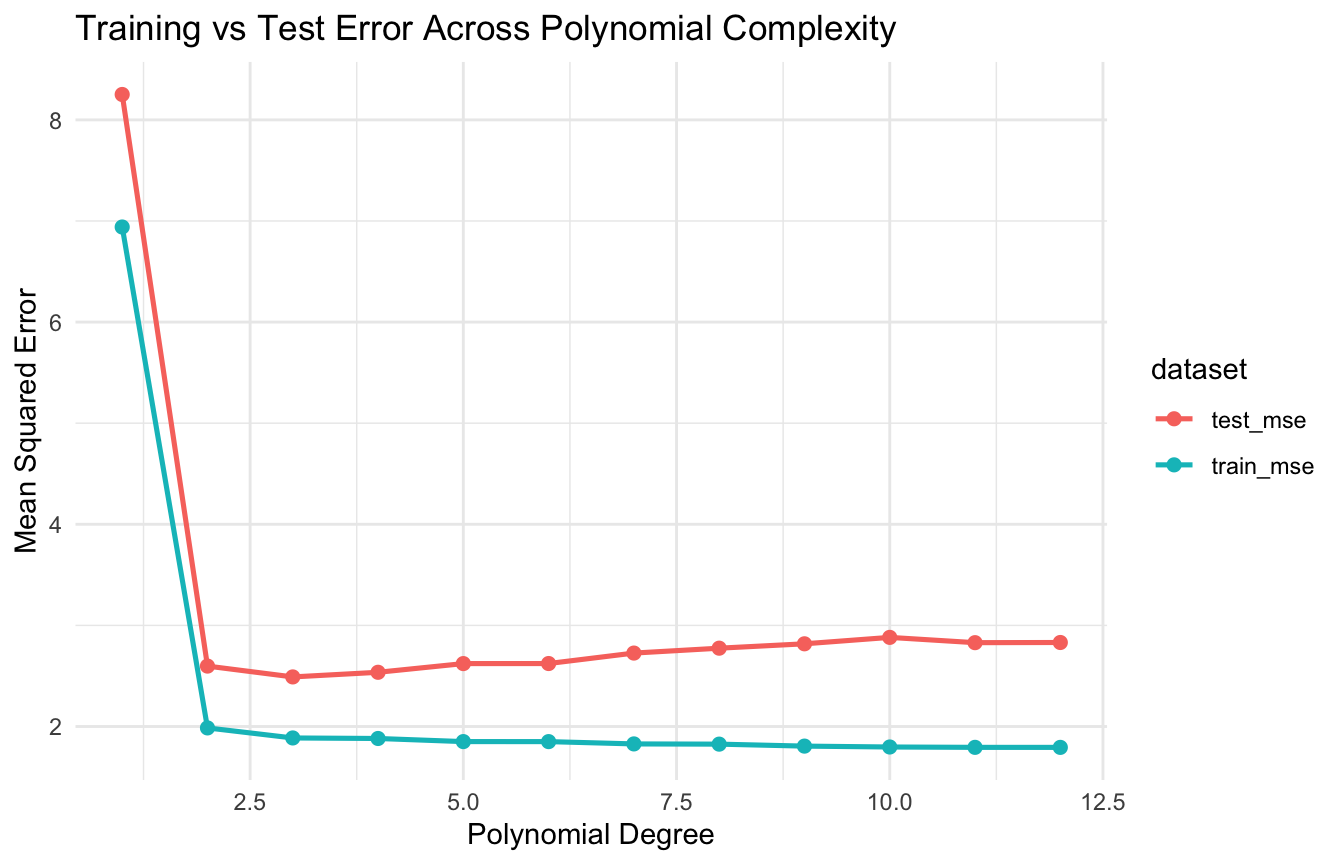
Mean Squared Error Is Where the Tradeoff Shows Up
A common way to summarize predictive error is mean squared error (MSE).
At a high level, prediction error can be thought of as having three components:
Regularization deliberately constrains a model to reduce variance.
This may increase bias slightly, but if the variance reduction is large enough, total prediction error can improve.
Examples include:
ridge regression
lasso
elastic net
early stopping
weight decay in neural networks
This is a central lesson in machine learning:
sometimes a slightly biased model predicts better because it is more stable.
Ensemble Methods Also Manage the Tradeoff
Another major response to the bias-variance problem is the use of ensembles.
Ensembles combine multiple models to improve predictive performance.
Different ensemble strategies affect bias and variance differently.
For example:
bagging and random forests often reduce variance
boosting often reduces bias, though it can also affect variance depending on tuning
This is one reason the bias-variance tradeoff is so important conceptually. It explains not only individual model behavior, but also why major algorithm families work the way they do.
High Bias and High Variance Require Different Fixes
A useful practical lesson is that not all poor performance should be fixed the same way.
If Bias Is High
The model may be too simple. Possible responses include:
adding features
increasing flexibility
allowing nonlinear terms
reducing regularization
If Variance Is High
The model may be too unstable. Possible responses include:
simplifying the model
adding regularization
increasing training data
using ensembles
reducing noise-sensitive predictors
This is why diagnosis matters. You cannot fix the right problem if you misidentify the failure mode.
The same tradeoff appears in many real models, including:
decision trees
random forests
boosting
splines
neural networks
nearest-neighbor models
penalized regressions
The language changes, but the central issue remains:
too rigid and you underfit
too flexible and you overfit
That is why the bias-variance tradeoff is one of the most portable ideas in modern analytics.
The Tradeoff Also Shapes Baseline Model Strategy
In practice, simpler baseline models are useful not only because they are interpretable, but also because they often have relatively low variance.
A simple model may underfit slightly, but it may still generalize surprisingly well if the signal is modest and the data are noisy.
This is why strong analysts do not begin by assuming that more complexity is automatically better.
The right question is:
does the additional flexibility improve out-of-sample performance enough to justify the added instability?
That is a bias-variance question.
There Is No Universal Best Model Complexity
One of the most important implications of the bias-variance tradeoff is that there is no universally optimal level of complexity.
The right balance depends on:
sample size
signal-to-noise ratio
predictor structure
task complexity
and the cost of error
A more flexible model may be ideal in a large, information-rich dataset. The same model may be disastrous in a smaller, noisier setting.
This is why model selection must be data- and problem-specific.
Cross-Validation Is One of the Best Practical Tools for Managing the Tradeoff
Because the tradeoff is about generalization, one of the best practical tools for managing it is cross-validation.
Cross-validation helps estimate how a model performs on unseen data.
This makes it useful for:
tuning model complexity
selecting regularization strength
comparing candidate models
detecting overfitting
In modern ML workflows, cross-validation is often the operational way the bias-variance tradeoff gets handled.
The principle is statistical. The workflow is computational.
A Practical Checklist for Applied Work
Before choosing or tuning a predictive model, ask:
Is the model underfitting or overfitting?
How do training and validation error compare?
Would more flexibility reduce bias or just increase variance?
Would regularization improve stability?
Would more data help close the generalization gap?
Are learning curves suggesting a persistent problem?
Is a simpler baseline already performing competitively?
These questions often improve model choice more than blind complexity escalation.
NoteWhere This Shows Up in AI/ML
Every ML model selection decision in clinical AI is a bias-variance decision: a gradient boosted tree with 500 estimators and deep interaction structure may achieve 0.91 AUC on DoDTR training data and 0.74 on prospective validation, while a regularized logistic regression achieves 0.83 on both — the gap is not noise, it is variance from overfitting to the trauma registry’s site-specific documentation patterns. Trauma mortality models are especially prone to this failure: injury severity scores, mechanism codes, and vitals are documented differently across Level I trauma centers versus far-forward MTFs, so a model trained on one context memorizes institutional artifacts that do not transfer. In deep learning, the double descent phenomenon means that very large models can actually escape the classical bias-variance tradeoff through overparameterization, but this requires massive datasets and careful regularization that are rarely present in military health registry settings. The operationally safe default is to select the simplest model whose out-of-sample performance is competitive, then require prospective validation before deployment.
Closing: Good Models Balance Fit with Stability
The bias-variance tradeoff remains one of the most important ideas in statistics and machine learning because it explains why prediction is not a one-dimensional optimization problem.
A model can fail by being too simple. It can also fail by being too unstable.
That is why good modeling is not about chasing the lowest training error. It is about balancing structure and restraint.
This is the logic behind:
regularization
ensemble methods
cross-validation
and thoughtful model selection
The bias-variance tradeoff matters because the best model is usually not the one that fits the hardest, but the one that generalizes with the right balance of flexibility and discipline.
This post is part of the Prediction Modeling Toolkit — a companion reference with learning curve diagnostics, regularization selection templates, and model complexity evaluation scaffolds.
Domingos, Pedro. 2000. “A Unified Bias-Variance Decomposition for Zero-One and Squared Loss.”Proceedings of the Seventeenth National Conference on Artificial Intelligence, 564–69.
Hastie, Trevor, Robert Tibshirani, and Jerome Friedman. 2009. The Elements of Statistical Learning: Data Mining, Inference, and Prediction. 2nd ed. Springer.
Hoerl, Arthur E., and Robert W. Kennard. 1970. “Ridge Regression: Biased Estimation for Nonorthogonal Problems.”Technometrics 12 (1): 55–67.
James, Gareth, Daniela Witten, Trevor Hastie, and Robert Tibshirani. 2021. An Introduction to Statistical Learning: With Applications in R. 2nd ed. Springer.
Tibshirani, Robert. 1996. “Regression Shrinkage and Selection via the Lasso.”Journal of the Royal Statistical Society: Series B 58 (1): 267–88.