Non-parametric methods aim to be more flexible by reducing dependence on rigid distributional forms. They are often attractive when the analyst wants to:
estimate structure from the data directly,
compare groups without assuming normality,
or quantify uncertainty without relying entirely on analytic formulas.
These methods matter in both statistics and AI/ML because they offer robustness, flexibility, and a useful alternative when assumptions become fragile.
Non-parametric methods matter because not all data deserve a rigid model, and sometimes the safest analysis begins by assuming less.
Non-Parametric Does Not Mean No Assumptions
A common misunderstanding is that “non-parametric” means assumption-free.
It does not.
Non-parametric methods still make assumptions. They simply avoid committing to a narrow parametric family like:
normal,
Poisson,
binomial,
or exponential.
For example:
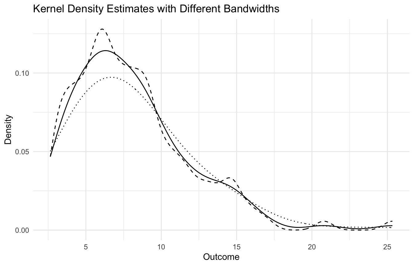
kernel density estimation assumes smoothness choices through bandwidth
rank tests assume meaningful ordering and certain independence conditions
bootstrap procedures assume the observed sample is informative enough to resample from
So the value of non-parametric methods is not that they eliminate assumptions. It is that they often replace strong structural assumptions with weaker or more flexible ones.
Parametric and Non-Parametric Thinking Solve Different Problems
A parametric model asks us to specify a family of distributions and estimate a finite number of parameters.
For example:
normal model: estimate mean and variance
logistic regression: estimate coefficients
Poisson model: estimate event rate
A non-parametric approach often asks a different question:
what can we learn from the observed data structure without forcing it into a narrow predefined shape?
That makes non-parametric methods especially appealing in exploratory analysis, robust comparison, and early-stage modeling.
This is also why they are often useful when data look messy, heterogeneous, or only partially aligned with textbook assumptions.
Kernel Density Estimation Is a Flexible Alternative to the Histogram
One of the simplest and most useful non-parametric tools is kernel density estimation, or KDE.
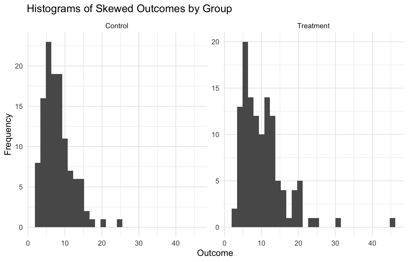
A histogram is often the first way analysts visualize a distribution. But histograms depend strongly on bin choice, and their shape can look jagged or unstable.
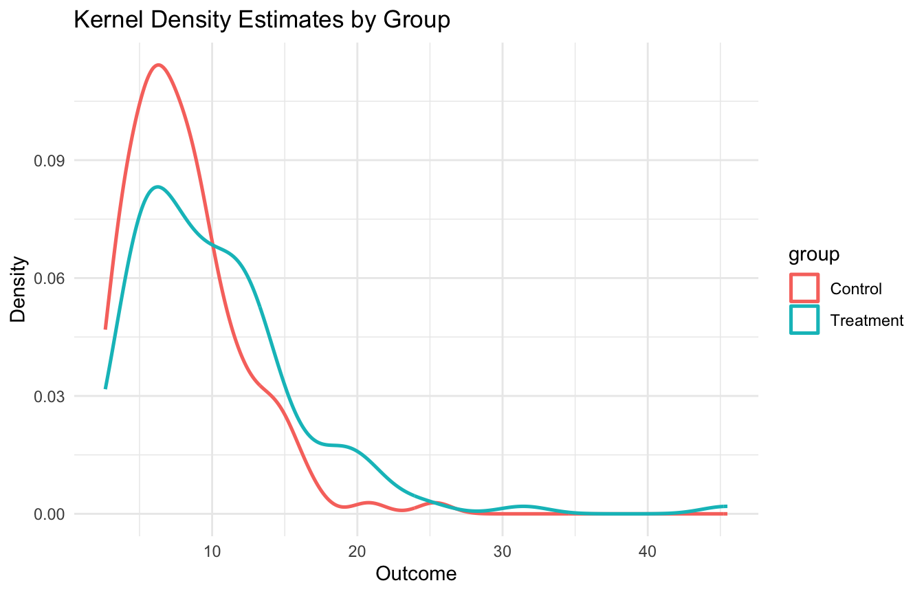
Kernel density estimation provides a smoother alternative.
The idea is simple:
place a small smooth bump around each observation and add them together.
This creates a continuous estimate of the distribution rather than a fixed-bin summary.
That makes KDE especially useful for visualizing:
skewness
multimodality
heavy tails
and group differences in distribution shape
A Biostats-Style Example Makes the Problem Concrete
To illustrate, we will simulate a continuous outcome with skew and heterogeneity.
Think of this as something like a biomarker, symptom burden, or recovery-related measure with a less-than-normal distribution.
This is a useful reminder that flexibility does not remove analyst responsibility.
Rank-Based Tests Compare Groups Without Assuming Normality
When comparing two groups, analysts often reach automatically for a t-test.
That may be fine when:
the outcome is roughly symmetric,
variances are reasonably stable,
and sample sizes are not tiny.
But when distributions are skewed or outlier-prone, a rank-based test can be attractive.
A common choice is the Wilcoxon rank-sum test, also known as the Mann-Whitney test.
This test works with the ranks of the data rather than the raw values themselves.
That makes it more robust to certain distributional problems.
The Wilcoxon / Mann-Whitney Test Is Often a Useful Alternative to the t-Test
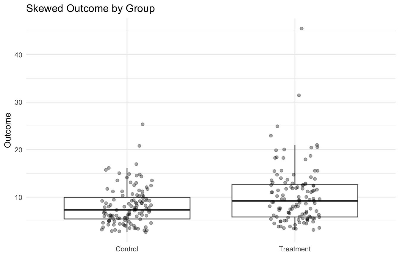
We can compare the two groups in the skewed dataset using both a classical t-test and a Wilcoxon test.
t_test_res <-t.test(outcome ~ group, data = np_df)wilcox_res <-wilcox.test(outcome ~ group, data = np_df)t_test_res
    Welch Two Sample t-test

data:  outcome by group
t = -3.4057, df = 203.08, p-value = 0.0007955
alternative hypothesis: true difference in means between group Control and group Treatment is not equal to 0
95 percent confidence interval:
 -3.5572895 -0.9485951
sample estimates:
  mean in group Control mean in group Treatment
               8.072221               10.325163
wilcox_res
    Wilcoxon rank sum test with continuity correction

data:  outcome by group
W = 5574, p-value = 0.002506
alternative hypothesis: true location shift is not equal to 0
These two tests answer slightly different inferential questions.
The t-test is oriented around mean differences under distributional assumptions. The Wilcoxon test is rank-based and is often interpreted as testing for a location shift under appropriate conditions (Mann and Whitney 1947; Lehmann and D’Abrera 2006).
This distinction matters. They are not interchangeable in every conceptual sense, even if they are often used for similar practical purposes.
Rank Tests Are Useful, but They Also Have Limits
Rank-based tests are robust in many settings, but they are not universally superior.
They can be especially useful when:
the data are skewed
the outcome is ordinal
outliers make mean-based inference unstable
distributional assumptions are dubious
But they also have limits.
For example:
they may be less directly tied to mean differences
they may lose interpretability when raw-scale effect size matters
they still rely on meaningful ranking and independence assumptions
So the right lesson is not “always use non-parametric tests.” It is “use them when their assumptions and inferential targets fit the problem better.”
Boxplots and Jittered Points Help Support Rank-Based Interpretation
Before and after formal testing, a visualization helps clarify what the test is reacting to.
This is a useful example because it shows how bootstrap methods can support inference for statistics that are less convenient to handle analytically.
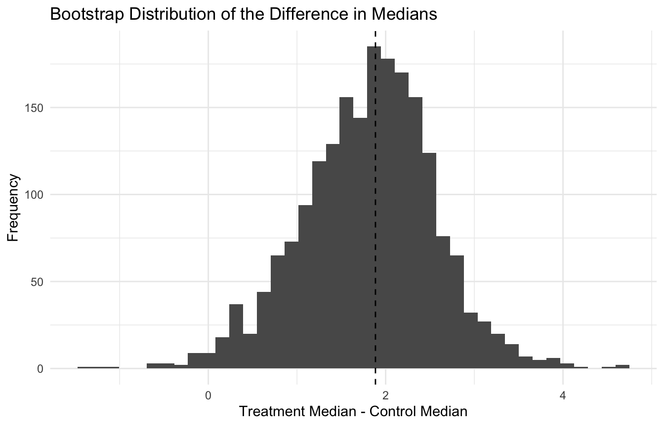
Bootstrap Distributions Make Uncertainty More Tangible
A major advantage of the bootstrap is that it makes the uncertainty of a statistic visible.
ggplot2::ggplot(boot_tbl, ggplot2::aes(x = diff_median)) + ggplot2::geom_histogram(bins =40) + ggplot2::geom_vline(xintercept =median(treat_vals) -median(control_vals), linetype =2) + ggplot2::labs(title ="Bootstrap Distribution of the Difference in Medians",x ="Treatment Median - Control Median",y ="Frequency" ) + ggplot2::theme_minimal()
This kind of plot helps communicate that estimation is not just about a point summary. It is about a distribution of plausible values.
Non-Parametric Thinking Is Also Important in AI/ML
Non-parametric methods are not just classical robust alternatives. They also matter in modern AI/ML.
Examples include:
kernel methods, such as support vector machines
density-based clustering
nearest-neighbor methods
bootstrap-based uncertainty assessment
flexible smoothing and local estimation ideas
These methods often avoid rigid parametric modeling of the full data distribution.
Instead, they let the data shape the structure more directly.
This is one reason non-parametric thinking remains central even in highly modern pipelines.
Kernel Ideas Extend Far Beyond Density Estimation
Kernel density estimation is only one member of a broader family of kernel-based ideas.
In AI/ML, kernels also appear in methods such as:
support vector machines
kernel PCA
local smoothing
Gaussian-process style covariance thinking
The central intuition is similar:
use localized similarity structure to build flexible models without forcing a rigid global form.
That is one reason KDE is pedagogically useful. It introduces a more general way of thinking about flexible modeling.
Comparing Parametric and Non-Parametric Approaches Is Often the Best Teaching Strategy
One of the most useful ways to understand non-parametric methods is to compare them directly with parametric alternatives.
For example:
histogram vs. fitted normal density
KDE vs. parametric distribution fit
t-test vs. Wilcoxon test
analytic interval vs. bootstrap interval
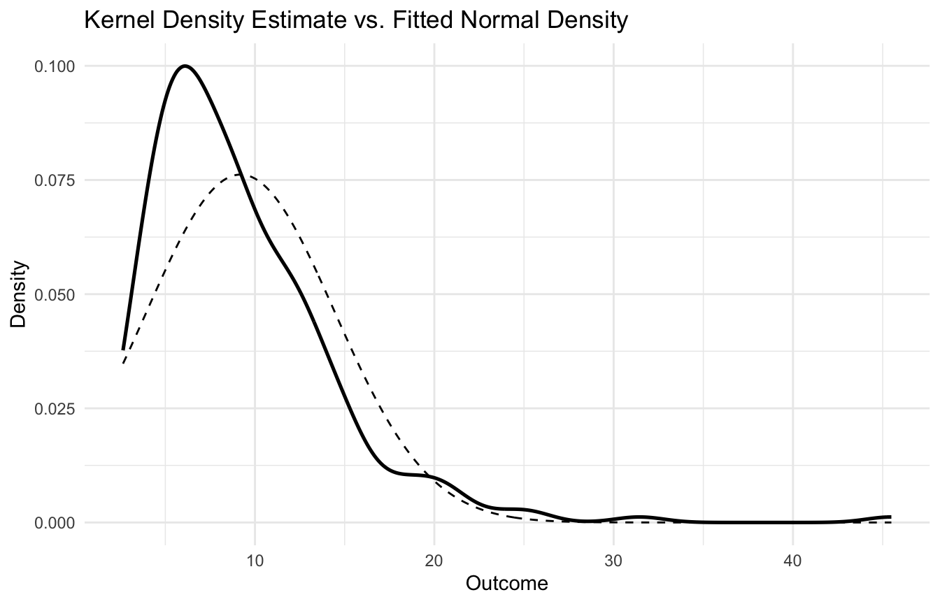
Below is a quick visual comparison of the observed skewed distribution with a fitted normal density.
overall_mean <-mean(np_df$outcome)overall_sd <-sd(np_df$outcome)x_grid <-seq(min(np_df$outcome), max(np_df$outcome), length.out =500)normal_overlay_df <- tibble::tibble(x = x_grid,density =dnorm(x_grid, mean = overall_mean, sd = overall_sd))ggplot2::ggplot(np_df, ggplot2::aes(x = outcome)) + ggplot2::geom_density(linewidth =0.9) + ggplot2::geom_line(data = normal_overlay_df, ggplot2::aes(x = x, y = density),linetype =2 ) + ggplot2::labs(title ="Kernel Density Estimate vs. Fitted Normal Density",x ="Outcome",y ="Density" ) + ggplot2::theme_minimal()
This type of comparison helps readers see why a flexible non-parametric approach may sometimes be preferable.
Non-Parametric Methods Are Often More Robust, but Sometimes Less Efficient
There is always a tradeoff.
When the parametric assumptions are approximately correct, parametric methods can be more statistically efficient.
But when those assumptions are poor, non-parametric methods can be more robust and more trustworthy.
That is one reason these methods are so useful in messy real-world settings.
The goal is not to choose one philosophy forever. It is to use the method whose assumptions and inferential target best fit the data problem.
Non-Parametric Does Not Mean “Exploratory Only”
Another misconception is that non-parametric methods are only informal exploratory tools.
That is false.
Many non-parametric methods support rigorous inference, estimation, and modeling.
Examples include:
formal rank-based tests
bootstrap confidence intervals
kernel density estimation
and several major ML methods built on local similarity or flexible structure
So non-parametric methods are not a fallback for weak analysis. They are a serious part of the statistical toolkit.
A Practical Checklist for Applied Work
Before choosing a non-parametric approach, ask:
Are the data strongly skewed, heavy-tailed, or outlier-prone?
Does the scientific question concern means, medians, ranks, or distribution shape?
Would a parametric model be interpretable and credible here?
Does a rank-based method better match the measurement scale?
Would bootstrap inference help quantify uncertainty more honestly?
Is the smoothing choice in KDE reasonable?
Am I choosing a non-parametric method because it fits the problem, or only because the parametric alternative is uncomfortable?
These questions usually lead to better analysis choices.
NoteWhere This Shows Up in AI/ML
Permutation testing is the standard for statistically rigorous model comparison in clinical AI validation: rather than assuming a parametric distribution for the difference in AUC between two models, analysts shuffle outcome labels and recompute the test statistic thousands of times to build an empirical null distribution. Bootstrap resampling is how confidence intervals for AUC are computed in FDA submissions for AI/ML-based software as a medical device — the percentile bootstrap CI is standard precisely because AUC does not have a simple closed-form sampling distribution under complex modeling scenarios. In DoDTR trauma outcome data, blood pressure, lactate, and ISS distributions are heavily skewed with long right tails from severe polytrauma cases; applying t-tests or ANOVA to raw values without transformation or rank-based alternatives produces p-values that reflect distributional artifacts as much as real group differences. The failure mode is not choosing the wrong test in isolation — it is reporting overly narrow confidence intervals from a normality assumption that the data clearly violate, creating false precision in a validation study.
Closing: Non-Parametric Methods Make Statistics More Flexible
Non-parametric methods remain important because real data often resist clean parametric assumptions.
Kernel density estimation helps reveal distributional shape without rigid forms. Rank-based tests provide robust alternatives for group comparison. Bootstrap inference offers flexible uncertainty quantification when formulas are inconvenient or fragile.
These ideas matter in both classical statistics and modern AI/ML because they encourage a more adaptable relationship between models and data.
Non-parametric methods matter because flexible data deserve flexible tools, especially when rigid assumptions would create more confidence than the evidence supports.
This post is part of the Prediction Modeling Toolkit — a companion reference with kernel density templates, rank-based test scaffolds, and bootstrap inference code for non-normal clinical outcomes.
Efron, Bradley, and Robert J. Tibshirani. 1994. An Introduction to the Bootstrap. Chapman; Hall/CRC.
Lehmann, E. L., and H. J. M. D’Abrera. 2006. Nonparametrics: Statistical Methods Based on Ranks. Springer.
Mann, Henry B., and Donald R. Whitney. 1947. “On a Test of Whether One of Two Random Variables Is Stochastically Larger Than the Other.”The Annals of Mathematical Statistics 18 (1): 50–60. https://doi.org/10.1214/aoms/1177730491.
Silverman, B. W. 1986. Density Estimation for Statistics and Data Analysis. Chapman; Hall.
Wasserman, Larry. 2004. All of Statistics: A Concise Course in Statistical Inference. Springer.