This matters not only in biostatistics, but also in AI/ML settings involving churn, event prediction, and lifetime modeling.
This post introduces:
censoring,
Kaplan-Meier curves,
hazard functions,
and Cox proportional hazards models,
with a clinical-trial style example.
Survival analysis matters because event timing contains information that ordinary yes/no outcomes throw away, and censoring means missing event times are often informative, not ignorable.
Survival Analysis Begins with Time-to-Event Thinking
In standard binary outcome analysis, we might ask whether an event happened.
In survival analysis, we ask something richer:
how long until the event occurs?
how does risk evolve over time?
do groups differ in their time-to-event patterns?
how do predictors affect the event hazard?
This shift matters because two patients can both experience the same event, but at very different times.
Time carries information.
That is why survival analysis is not just a niche add-on to regression. It is the natural framework for studying event timing.
Censoring Is the Central Data Challenge
One of the defining features of survival data is censoring.
Right censoring occurs when:
a subject has not yet experienced the event by the end of follow-up,
is lost to follow-up,
or leaves observation before the event occurs.
In these cases, we do not know the exact event time. We only know that it exceeds the observed follow-up time.
That is critically different from ordinary missing data.
A censored observation still provides partial information. It tells us the subject survived or remained event-free up to a known time.
Survival methods are designed to use that partial information correctly.
The Survival Function and Hazard Function Capture Different Ideas
Two fundamental quantities in survival analysis are:
Survival Function
\[
S(t) = P(T > t)
\]
This is the probability that the event time (T) exceeds time (t).
It answers:
what proportion remain event-free beyond time (t)?
Hazard Function
The hazard describes the instantaneous event risk at time (t), given survival up to that point.
Very loosely, it answers:
among those still at risk, how likely is the event to occur next?
The survival function is often easier to visualize. The hazard function is often more natural for modeling covariate effects.
Both are central.
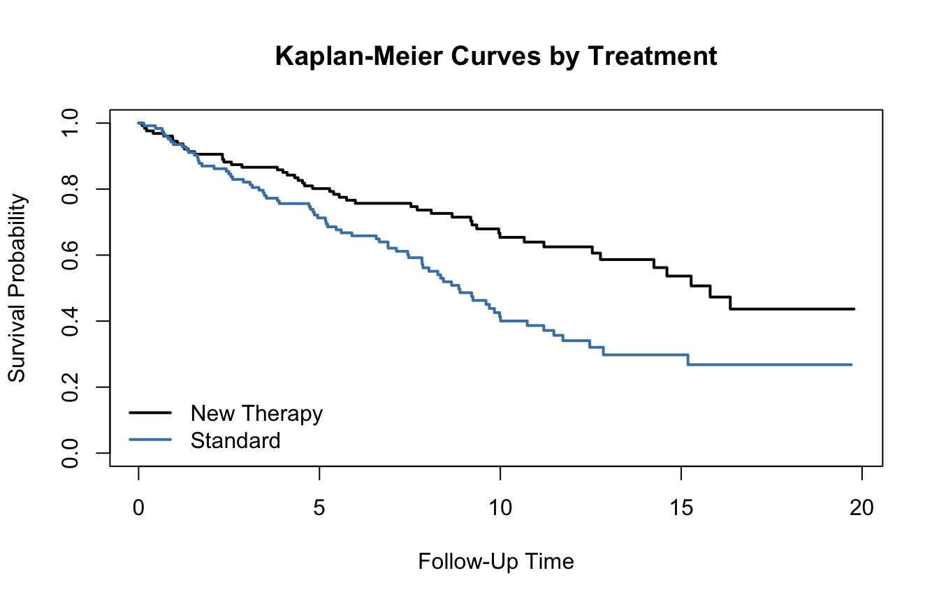
A Clinical-Trial Style Example Makes the Problem Concrete
To illustrate survival analysis, we will simulate a simple clinical-trial style dataset with:
# A tibble: 2 × 3
  term              estimate hazard_ratio
  <chr>                <dbl>        <dbl>
1 treatmentStandard   0.646          1.91
2 age                 0.0200         1.02
Interpretation example:
a hazard ratio below 1 for New Therapy suggests lower event hazard than the reference group
a hazard ratio above 1 for age suggests that higher age is associated with increased hazard
This is a conditional interpretation:
treatment effect holding age constant
age effect holding treatment constant
That is one of the strengths of the Cox model compared with simple curve comparison alone.
The Cox Model Is About Hazard, Not Directly About Survival Time
One of the most common interpretive pitfalls is to treat hazard ratios as if they were simple ratios of survival times.
They are not.
A hazard ratio is a ratio of instantaneous event rates among those still at risk.
That makes it very useful, but also more subtle than a direct “time multiplier.”
In practice, this means:
hazard ratios are informative,
but they should not be oversimplified into claims about exact survival duration differences.
The hazard framing is one of the reasons survival analysis requires careful language.
The Proportional Hazards Assumption Must Be Checked
A central assumption of the Cox model is proportional hazards(Cox 1972).
This means the hazard ratio between groups is assumed to remain constant over time.
If this assumption is badly violated, the model may become misleading.
A standard diagnostic uses Schoenfeld residuals.
survival::cox.zph(fit_cox)
          chisq df    p
treatment 0.632  1 0.43
age       0.375  1 0.54
GLOBAL    0.915  2 0.63
This test and its associated plots help assess whether the proportional hazards assumption is reasonable.
In applied work, this is not optional bookkeeping. It is part of responsible interpretation.
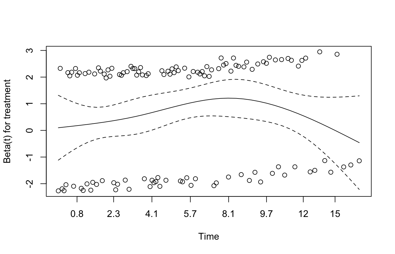
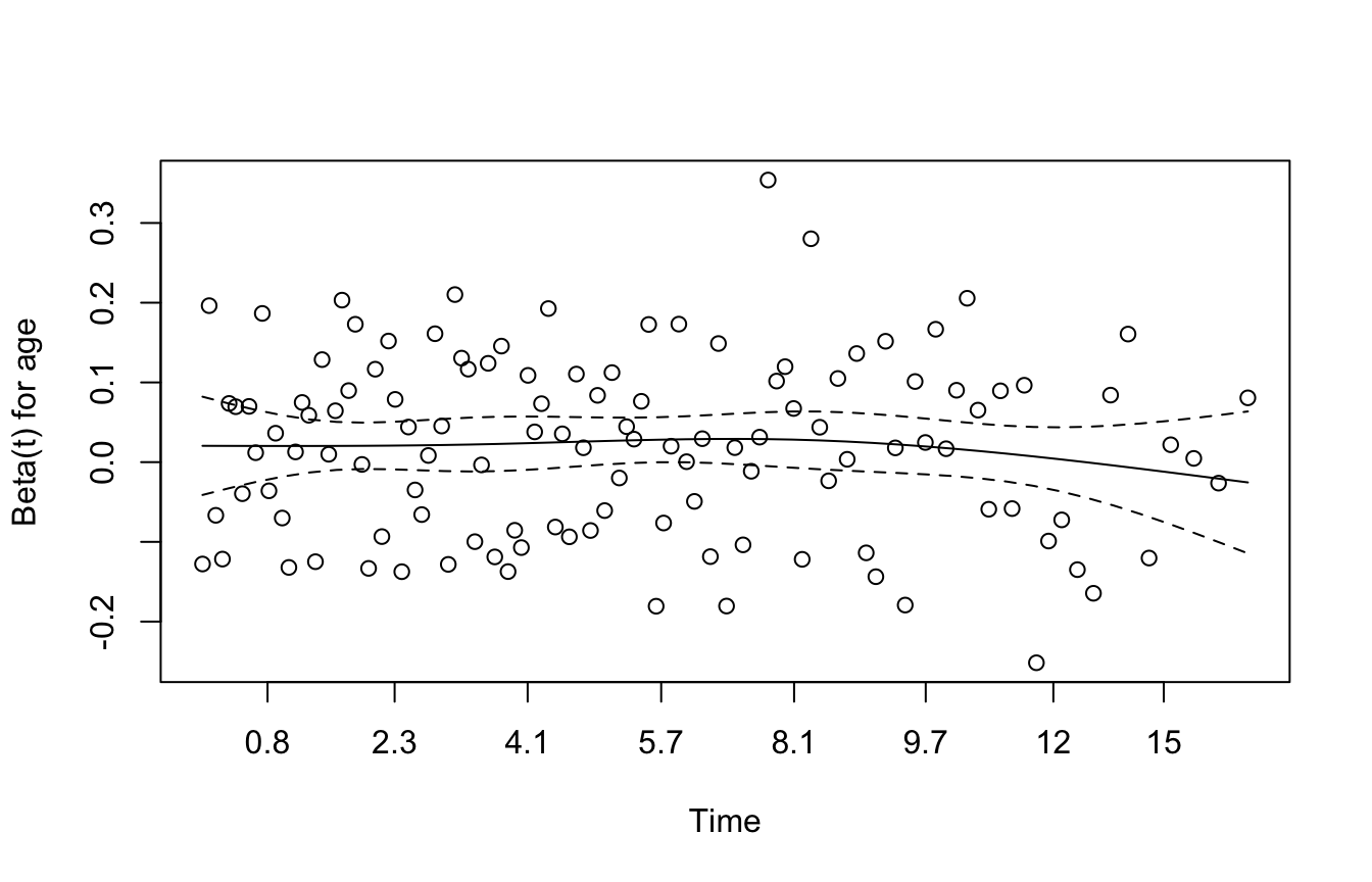
Visual Diagnostics Help Assess Proportionality
If you want a graphical check, you can plot the proportional hazards diagnostics.
plot(survival::cox.zph(fit_cox))
If the effect appears to vary strongly over time, then the proportional hazards assumption may be questionable.
In such cases, analysts may need:
time-varying effects
stratified Cox models
or alternative survival modeling approaches
This is one reason survival analysis remains a modeling discipline, not merely a software routine.
Survival Analysis Matters in AI/ML Because Many Events Are Time-Dependent
Survival analysis is not confined to clinical trials.
It also matters in AI/ML settings such as:
churn prediction
customer lifetime analysis
equipment failure forecasting
retention modeling
time-to-conversion problems
and maintenance scheduling
In all of these problems, the key issue is not only whether an event occurs, but when.
That is why survival methods remain important even as more ML approaches emerge.
They handle event timing and censoring directly, which many naïve classifiers do not.
Survival ML Extends Classical Ideas Rather Than Replacing Them
Modern ML has produced extensions such as:
random survival forests
penalized Cox models
deep survival models
and neural hazard-based approaches
But these do not make classical survival analysis obsolete.
Instead, they build on the same central concerns:
censoring
time-to-event structure
hazard or survival estimation
and temporal risk prediction
That is why learning Kaplan-Meier and Cox PH still matters. They remain the conceptual foundation for many survival-oriented ML methods.
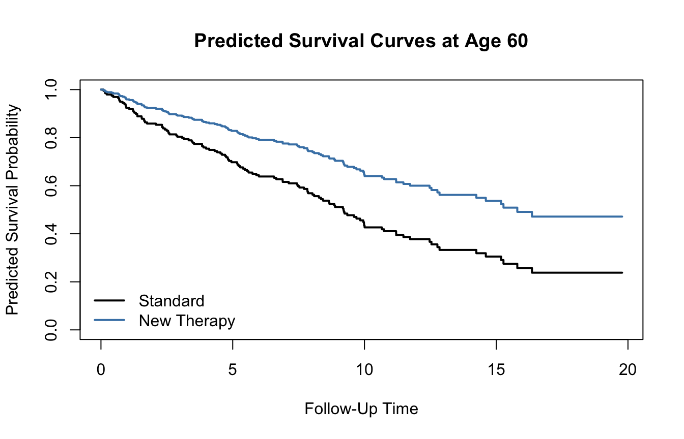
A Predicted Survival Curve Can Be More Intuitive Than a Hazard Ratio Alone
One useful feature of the Cox model is that it can be used to generate survival curves for specific covariate patterns.
newdata_df <-data.frame(treatment =c("Standard", "New Therapy"),age =c(60, 60))pred_surv <- survival::survfit(fit_cox, newdata = newdata_df)plot( pred_surv,col =c("black", "steelblue"),lwd =2,xlab ="Follow-Up Time",ylab ="Predicted Survival Probability",main ="Predicted Survival Curves at Age 60")legend("bottomleft",legend =c("Standard", "New Therapy"),col =c("black", "steelblue"),lwd =2,bty ="n")
This is often easier for readers to understand than hazard ratios alone, especially when communicating to non-statistical audiences.
Survival Analysis Is About More Than Significance
As with many classical methods, survival analysis can be reduced too quickly to p-values.
That misses much of what makes it useful.
Survival analysis is valuable because it provides:
time-aware estimation
use of censored data
interpretable risk modeling
and clinically or operationally meaningful curves
A significant hazard ratio is only part of the story.
The more important questions often are:
how large is the effect?
when do the curves diverge?
how much censoring is present?
and does the model fit the temporal structure credibly?
That is where good analysis lives.
A Practical Checklist for Applied Work
Before reporting a survival analysis, ask:
Is the event clearly defined?
Is censoring being handled properly?
Have I plotted Kaplan-Meier curves?
Is group comparison enough, or is covariate adjustment needed?
Are hazard ratios being interpreted correctly?
Has the proportional hazards assumption been checked?
Would predicted survival curves help communication?
Is a more flexible survival ML approach justified, or is a classical model already adequate?
These questions often matter more than whether the software output looks polished.
NoteWhere This Shows Up in AI/ML
Time-to-event modeling drives readmission prediction, post-discharge mortality surveillance, and medical device failure forecasting across deployed health systems: Epic’s readmission risk model is structurally a competing risks survival problem, since patients can be readmitted, die, or be administratively censored, and treating all non-readmission as equivalent obscures which failure mode dominates. Standard binary classifiers applied to censored survival outcomes produce biased estimates because they discard information from patients who haven’t yet experienced the event — a patient censored at 25 days is not the same as a patient who was event-free at 90 days, but a logistic model treats them identically if both are coded “0.” In DoDTR trauma cohorts, competing risks are pervasive: a service member who dies in the first 48 hours cannot experience a 30-day infectious complication, and standard Cox models that ignore this competing event will overestimate cumulative complication incidence in high-mortality subgroups. Applying a single-event Cox model in this setting inflates complication risk estimates and can lead to over-aggressive prophylaxis protocols.
Closing: Survival Analysis Keeps Time and Uncertainty in the Same Model
Survival analysis remains one of the most important areas of applied statistics because it handles two realities at once:
events take time,
and follow-up is often incomplete.
Kaplan-Meier curves offer a transparent way to estimate survival probabilities. Cox models allow covariate-adjusted hazard modeling without fully specifying the baseline hazard. Together, they provide a powerful framework for event-time data in both biostatistics and AI/ML.
Survival analysis matters because timing is data, censoring is not failure, and understanding event risk over time is central to many real decisions.
This post is part of the Survival Analysis Toolkit — a companion reference with Kaplan-Meier templates, Cox model diagnostics, censoring documentation standards, and time-to-event reporting scaffolds.
Kaplan, Edward L., and Paul Meier. 1958. “Nonparametric Estimation from Incomplete Observations.”Journal of the American Statistical Association 53 (282): 457–81. https://doi.org/10.1080/01621459.1958.10501452.
Klein, John P., and Melvin L. Moeschberger. 2003. Survival Analysis: Techniques for Censored and Truncated Data. 2nd ed. Springer.