A practical introduction to time series analysis, stationarity, ARIMA models, forecasting, and diagnostics for AI and clinical decision-making.
Published
July 15, 2024
Modified
June 9, 2026
Executive Summary
Many datasets are not just collections of independent observations.
They unfold over time.
That changes everything.
When data are ordered in time, the past can influence the future. Observations close together may be more similar than observations far apart. Trends, seasonality, shocks, and persistence all begin to matter.
The analyst must account for temporal dependence, not merely average relationships.
A Time Series Is About Dependence Across Time
A time series can be thought of as a sequence:
\[
Y_1, Y_2, Y_3, \dots, Y_T
\]
where each value is indexed by time.
The key idea is that these values are not arbitrary neighbors. Their ordering matters.
Time dependence can show up through:
trend, where the series drifts upward or downward
seasonality, where the series repeats cyclical patterns
autocorrelation, where past values help predict future values
volatility changes, where uncertainty itself varies over time
Understanding these patterns is the first step in any time series workflow.
Stationarity Is One of the Core Ideas
One of the most important concepts in time series analysis is stationarity.
A stationary process is one whose statistical properties are stable over time.
In broad applied terms, this often means:
the mean does not drift systematically,
the variance is roughly stable,
and the dependence structure is not changing unpredictably across time.
Why does this matter?
Because many classical time series models, including ARIMA components, work best when the underlying series is stationary or has been transformed into something close to stationary.
A nonstationary series often contains trend or other structure that must be handled before modeling dependence properly.
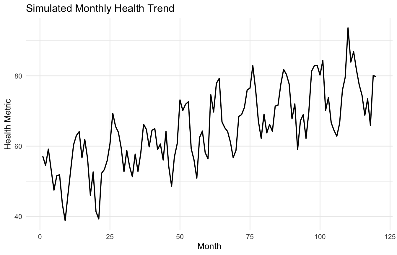
A Health-Trend Example Makes the Problem Concrete
To keep the example practical, we will simulate a simple monthly health-trend series, such as infection counts, clinic demand, or symptom burden over time.
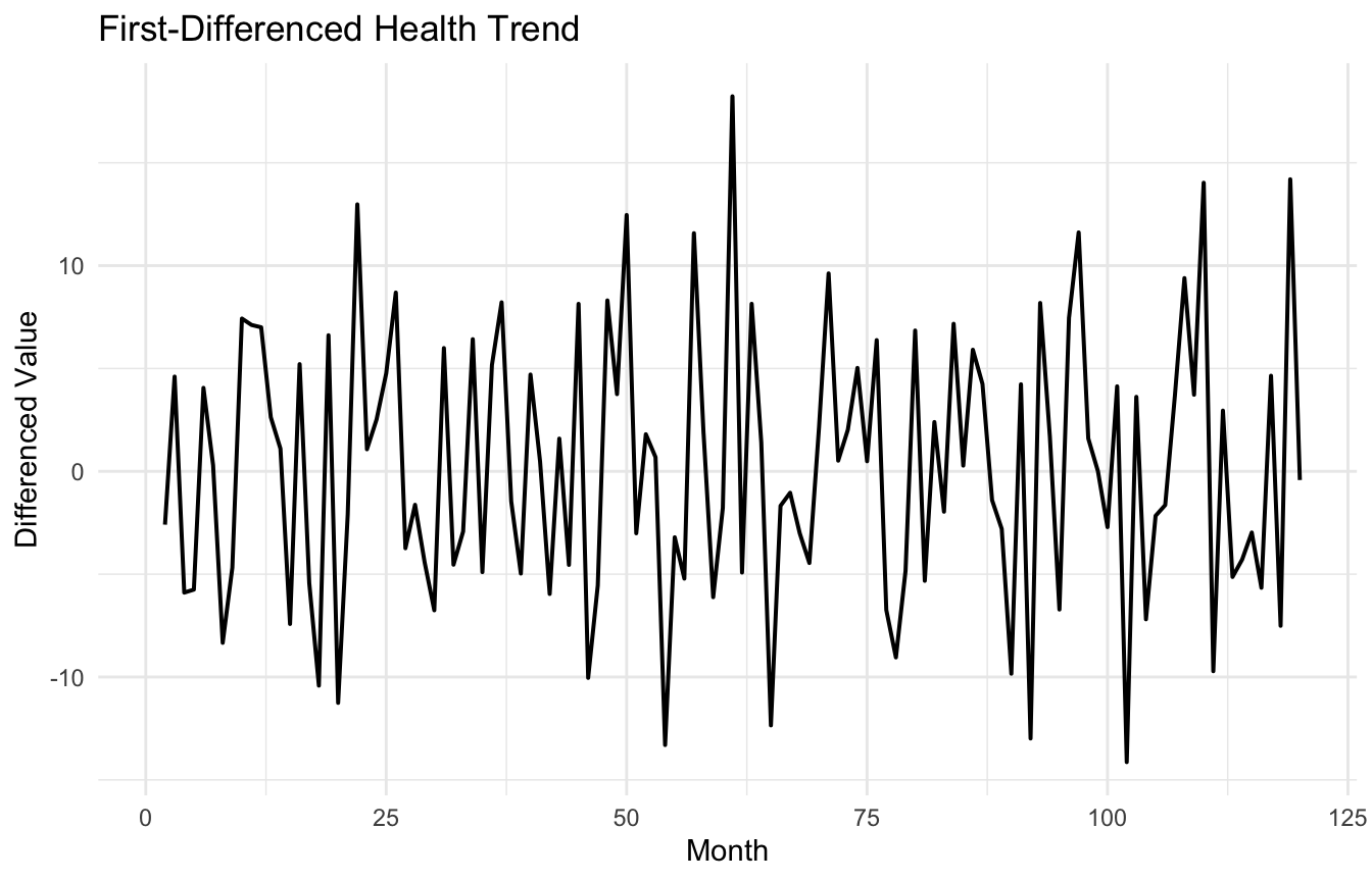
This is one of the most important classical forecasting frameworks because it handles:
nonstationarity through differencing
serial dependence through AR and MA structure
That makes ARIMA a powerful baseline time series model.
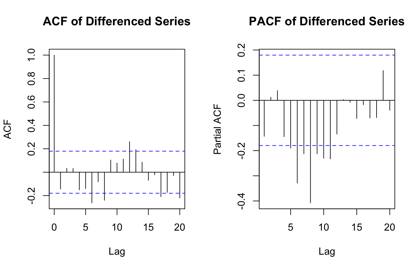
Autocorrelation Plots Help Suggest Model Structure
Two classic tools in time series diagnostics are:
the autocorrelation function (ACF)
the partial autocorrelation function (PACF)
These help suggest whether AR or MA structure may be present.
par(mfrow =c(1, 2))acf(na.omit(ts_df$diff_health_metric), main ="ACF of Differenced Series")pacf(na.omit(ts_df$diff_health_metric), main ="PACF of Differenced Series")
par(mfrow =c(1, 1))
In applied workflows, these plots are used heuristically.
They do not mechanically determine the right model, but they provide useful clues about the temporal dependence structure.
Fitting an ARIMA Model in R
We can fit an ARIMA model directly using arima() or forecast::Arima().
Below is a simple example.
fit_arima <-arima(ts_df$health_metric, order =c(1, 1, 1))fit_arima
Automated selection can be convenient, but it should not replace understanding.
A model chosen by information criteria is still only as useful as:
the assumptions behind it
the time structure in the data
and the forecasting context
Automation is helpful. Interpretation still matters.
Forecasting Requires Uncertainty, Not Just Point Predictions
One of the main goals of time series modeling is forecasting.
But a forecast is not just a future point estimate. It is also an uncertainty statement.
That is why forecast plots usually include:
a central forecast line
and confidence bands around it
These bands widen as the forecast horizon increases because uncertainty accumulates.
ts_obj <-ts(ts_df$health_metric, frequency =12)fit_auto <- forecast::auto.arima(ts_obj)fc <- forecast::forecast(fit_auto, h =12)plot(fc)
This is one of the places where classical statistics remains especially valuable: it forces uncertainty back into future predictions.
Forecast Confidence Bands Are a Guard Against False Precision
Forecast intervals are essential because future uncertainty is often larger than users expect.
Without uncertainty bands, a forecast can look falsely exact.
This is especially dangerous in:
health systems planning
staffing forecasts
supply chain projections
operational readiness estimates
financial or market trend communication
A point forecast says what is most plausible under the model. The confidence band reminds us how uncertain that future still is.
This is one of the key lessons time series analysis shares with the broader statistical tradition.
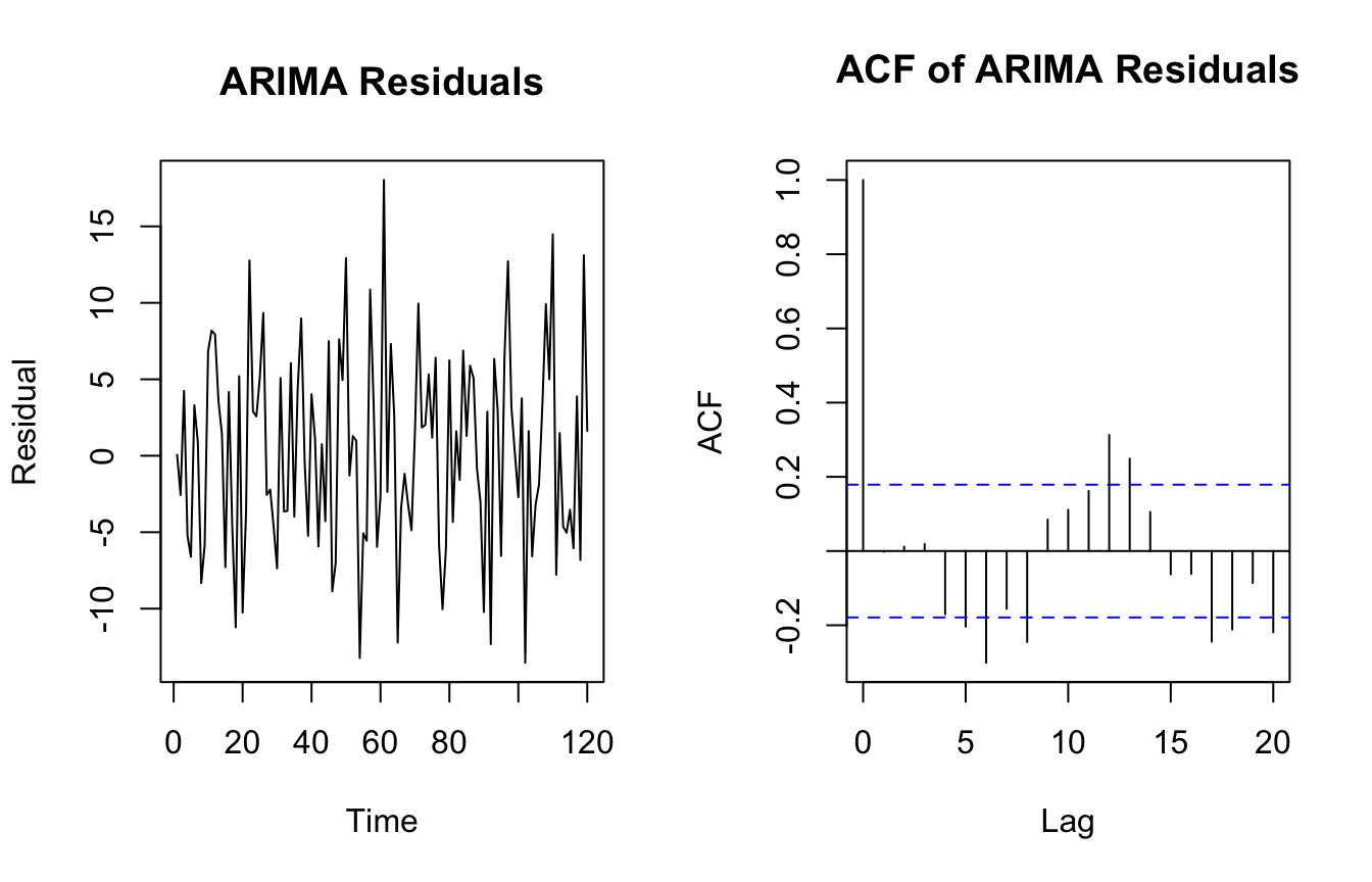
Residual Diagnostics Still Matter After Model Fitting
A fitted ARIMA model should leave residuals that look approximately like white noise.
That means the model should have captured most of the systematic time dependence.
Residual checks often include:
residual plots
residual ACF
Ljung-Box style tests for remaining autocorrelation
ts_resid <-residuals(fit_arima)par(mfrow =c(1, 2))plot(ts_resid, type ="l", main ="ARIMA Residuals", ylab ="Residual")acf(ts_resid, main ="ACF of ARIMA Residuals")
par(mfrow =c(1, 1))
If substantial autocorrelation remains, the model may be missing important temporal structure.
Time Series Methods Matter in AI/ML Because Sequence Matters
Modern AI/ML systems often work with sequential data:
physiological monitoring streams
stock prices
web traffic
wearable sensor data
device telemetry
language tokens
temporal event logs
What classical time series methods teach is not obsolete in these contexts.
They teach:
dependence across time
the importance of temporal ordering
the need for stationarity or transformation
and the distinction between signal and sequential noise
Even complex sequence models such as RNNs and LSTMs still live in the world of temporal dependence that classical time series analysis helped formalize.
ARIMA Is Not the Whole Story, but It Is a Powerful Baseline
ARIMA is not the only time series tool.
It does not automatically handle:
complex nonlinear structure
rich external covariates
regime switching
high-dimensional multivariate dependencies
or all seasonal complexities without extension
But it remains extremely valuable because it is:
interpretable
well understood
fast to fit
and often surprisingly competitive as a forecasting baseline
In ML practice, a strong classical baseline is always valuable. If a much more complex model does not clearly outperform it, that is meaningful.
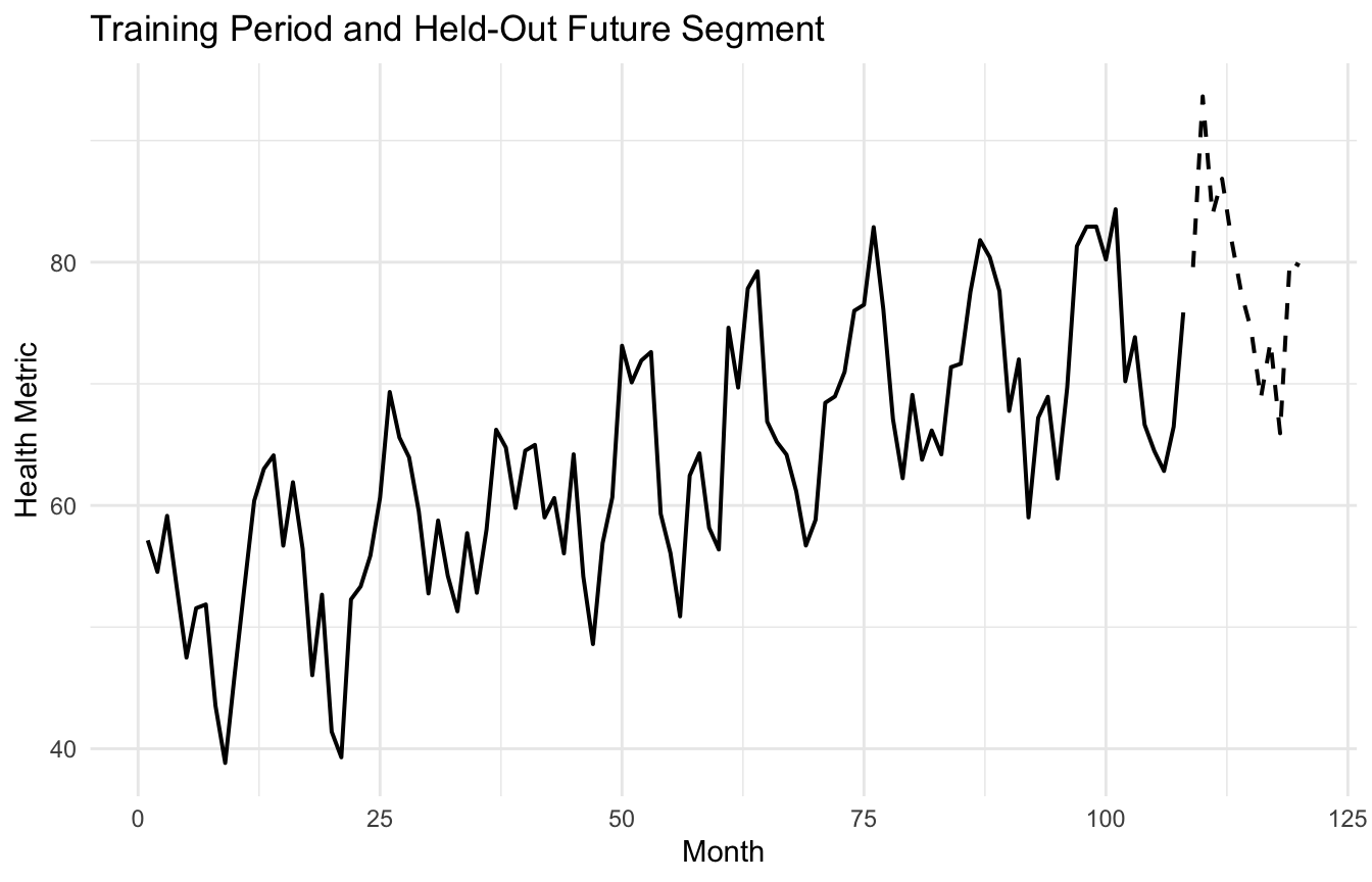
A Health-Trend Plot with a Simple Forecast Illustration
A useful final visualization is to split the series into training and future periods and show a basic forecast conceptually.
This kind of plot helps reinforce that forecasting should be evaluated on future-like data, not only on in-sample fit.
A Practical Checklist for Applied Work
Before fitting or reporting a time series model, ask:
Is the series approximately stationary, or does it need transformation?
Is there visible trend or seasonality?
Have I plotted the data before modeling?
Do ACF and PACF suggest meaningful dependence structure?
Are residuals approximately white noise after fitting?
Am I reporting forecast uncertainty, not just point forecasts?
Is ARIMA a sensible baseline before moving to more complex sequential models?
Does the model reflect the real forecasting use case?
These questions usually improve both rigor and communication.
NoteWhere This Shows Up in AI/ML
ICU early warning systems — including the sepsis prediction models deployed in Epic and Cerner — depend on time-series vital sign streams: each new observation inherits context from the preceding hours, and deterioration signals often emerge from trajectory rather than from any single value. LSTM and Transformer-based models for clinical early warning are architecturally designed to capture exactly this temporal dependency, treating each patient encounter as a sequence rather than an independent cross-section. The failure mode is using a static logistic regression model trained on admission-snapshot features to predict 24-hour deterioration in patients already in the ICU: the model sees where the patient started, not where the trajectory is heading, and systematically misses patients who deteriorate rapidly from an initially stable baseline. In military far-forward care, where vital signs may be recorded at irregular intervals under austere conditions, standard time-series assumptions about regular sampling intervals break down and must be explicitly addressed before applying ARIMA or LSTM-based approaches.
Closing: Time Series Analysis Teaches Statistical Respect for Time
Time series analysis matters because time introduces structure that ordinary methods cannot ignore.
AR, MA, and ARIMA models help analysts think clearly about:
dependence
stationarity
forecasting
and uncertainty over time
They remain valuable in their own right, and they also provide a conceptual foundation for more advanced AI/ML methods built for sequential data.
Time series methods still matter because predicting the future is not only about fitting patterns, but about respecting how the past shapes the present and constrains the future.
This post is part of the Real-World Evidence Toolkit — a companion reference with temporal data modeling templates, stationarity diagnostics, ARIMA scaffolds, and interrupted time series analysis code.