Clustering Secrets: Grouping Data Like a Pro in ML

Applied Statistics
Clustering
An applied introduction to clustering, K-means, hierarchical clustering, silhouette scores, and subgroup discovery in unsupervised learning.
Published

June 15, 2024

Modified

June 9, 2026

Executive Summary

Many datasets do not arrive with clear labels.

Instead of knowing ahead of time who belongs to which group, analysts are often confronted with a harder question:

Are there natural groupings hidden in the data?

That is the central problem of clustering.

Cluster analysis is one of the core tools of unsupervised learning (MacQueen 1967; Ward 1963; Hastie et al. 2009). It helps identify observations that look similar to one another and different from the rest.

In practice, clustering can be used for:

  • patient phenotyping,
  • customer segmentation,
  • anomaly exploration,
  • subgroup discovery,
  • and feature engineering before supervised modeling.

This matters in both biostatistics and AI/ML.

In biostatistics, clustering can reveal clinically meaningful patient profiles. In machine learning, clustering can support exploratory analysis, representation learning, and preprocessing for later predictive tasks.

This post introduces:

  • K-means clustering,
  • hierarchical clustering,
  • choosing the number of clusters,
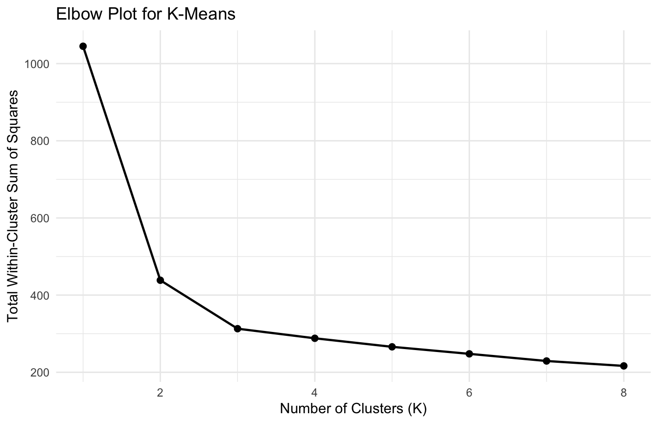
  • elbow plots,
  • silhouette scores,
  • and interpretation using a biostats-style patient-profile dataset.

Clustering matters because not every important pattern comes with a label, and learning to detect structure without supervision is one of the most useful skills in applied analytics.


Clustering Is About Discovering Structure Without Outcomes

Unlike regression or classification, clustering does not start with a known target variable.

There is no outcome to predict.

Instead, clustering asks whether the observations themselves contain meaningful structure.

That makes clustering fundamentally unsupervised.

This is important because many real datasets contain heterogeneity that is not explicitly labeled.

Examples include:

  • subtypes of patients with different physiologic patterns,
  • operational workflows that behave differently across contexts,
  • hidden user groups in digital platforms,
  • or biologic profiles that reflect distinct latent states.

Clustering is often the first step toward discovering those patterns.


Similarity Is the Hidden Foundation of Clustering

All clustering methods rely on a notion of similarity or dissimilarity (Kaufman and Rousseeuw 1990; Hastie et al. 2009).

At a practical level, clustering algorithms are asking:

  • which observations are close together?
  • which are far apart?
  • and how should that closeness be translated into groups?

This means clustering depends heavily on:

  • variable selection,
  • scaling,
  • distance metric,
  • and the clustering algorithm itself.

There is no cluster analysis without a definition of similarity.

That is why preprocessing decisions often matter as much as the clustering method.


Standardization Usually Matters Before Clustering

If one variable is measured on a much larger scale than another, it can dominate the distance calculation.

For example:

  • age may range from 18 to 90
  • lactate may range from 0 to 10
  • heart rate may range from 40 to 180

Without scaling, variables with larger numeric spread can overwhelm the clustering solution.

That is why standardization is often essential (Hastie et al. 2009; James et al. 2021).

In many applied settings, clustering should be performed on centered and scaled variables unless there is a strong reason not to.

This is especially important in biostats-style patient profiling, where features often come from different physiologic scales.


A Patient-Profile Example Makes the Task Concrete

To illustrate clustering, we will simulate a small patient-profile dataset with several continuous variables.

The example is synthetic, but it reflects a realistic applied idea: patients may cluster into profiles based on physiology and severity-related patterns.

library(dplyr)
library(tibble)
library(ggplot2)

n_per_group <- 70

cluster_df <- tibble::tibble(
  patient_id = 1:(3 * n_per_group),
  latent_group = rep(c("Profile A", "Profile B", "Profile C"), each = n_per_group),
  age = c(
    rnorm(n_per_group, mean = 35, sd = 6),
    rnorm(n_per_group, mean = 60, sd = 8),
    rnorm(n_per_group, mean = 48, sd = 7)
  ),
  heart_rate = c(
    rnorm(n_per_group, mean = 88, sd = 8),
    rnorm(n_per_group, mean = 102, sd = 10),
    rnorm(n_per_group, mean = 76, sd = 7)
  ),
  sbp = c(
    rnorm(n_per_group, mean = 122, sd = 10),
    rnorm(n_per_group, mean = 98, sd = 12),
    rnorm(n_per_group, mean = 135, sd = 9)
  ),
  lactate = c(
    rnorm(n_per_group, mean = 1.8, sd = 0.4),
    rnorm(n_per_group, mean = 4.5, sd = 0.8),
    rnorm(n_per_group, mean = 2.6, sd = 0.5)
  ),
  severity = c(
    rnorm(n_per_group, mean = 8, sd = 2),
    rnorm(n_per_group, mean = 16, sd = 3),
    rnorm(n_per_group, mean = 11, sd = 2)
  )
)

cluster_df |>
  dplyr::group_by(latent_group) |>
  dplyr::summarise(
    dplyr::across(
      c(age, heart_rate, sbp, lactate, severity),
      mean
    ),
    .groups = "drop"
  )
# A tibble: 3 × 6
  latent_group   age heart_rate   sbp lactate severity
  <chr>        <dbl>      <dbl> <dbl>   <dbl>    <dbl>
1 Profile A     34.8       89.4 121.     1.79     7.79
2 Profile B     60.0      103.   94.9    4.51    16.0 
3 Profile C     46.8       76.6 133.     2.65    11.5 

In real analysis, the latent grouping would be unknown. Here it exists only so we can see whether the clustering recovers meaningful structure.


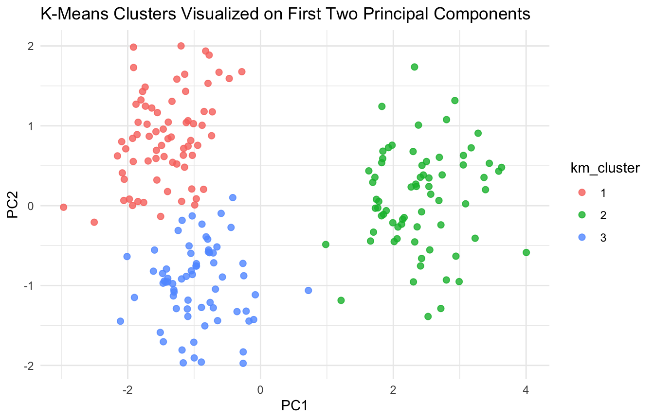
K-Means Clustering Partitions the Data Into K Groups

K-means is one of the most widely used clustering algorithms.

Its goal is simple:

partition the observations into (K) clusters so that observations within a cluster are as similar as possible, and observations across clusters are as different as possible.

K-means works by minimizing the within-cluster sum of squares.

That means it is trying to create compact clusters around cluster centroids.

Before fitting K-means, we standardize the features.

x_mat <- cluster_df |>
  dplyr::select(age, heart_rate, sbp, lactate, severity) |>
  scale()

Now fit a K-means solution with (K = 3).

km_fit <- kmeans(x_mat, centers = 3, nstart = 25)

cluster_df <- cluster_df |>
  dplyr::mutate(
    km_cluster = factor(km_fit$cluster)
  )

table(cluster_df$km_cluster)

 1  2  3 
72 70 68 

The nstart = 25 argument is important because K-means can depend on random starting values.


K-Means Is Fast and Useful, but It Assumes Compact Clusters

K-means is popular because it is:

  • simple,
  • fast,
  • and often effective in practice.

But it has assumptions built into it.

K-means works best when clusters are roughly:

  • spherical,
  • compact,
  • and separated in Euclidean space.

It is less well suited when clusters are:

  • strongly overlapping,
  • elongated,
  • nonlinear in shape,
  • or defined by more complex geometry.

This is one reason clustering should always be treated as an exploratory method rather than a guaranteed truth-discovery engine.


The Elbow Method Helps Choose K

A major practical question in K-means is: how many clusters should we choose?

One common heuristic is the elbow method.

The idea is to fit K-means for multiple values of (K) and track the total within-cluster sum of squares.

As (K) increases, within-cluster variability will always decrease. But after some point, the improvement may level off.

That point of diminishing returns is the “elbow.”

elbow_df <- tibble::tibble(
  k = 1:8,
  tot_withinss = purrr::map_dbl(
    1:8,
    ~ kmeans(x_mat, centers = .x, nstart = 25)$tot.withinss
  )
)

ggplot2::ggplot(elbow_df, ggplot2::aes(x = k, y = tot_withinss)) +
  ggplot2::geom_line(linewidth = 0.8) +
  ggplot2::geom_point(size = 2) +
  ggplot2::labs(
    title = "Elbow Plot for K-Means",
    x = "Number of Clusters (K)",
    y = "Total Within-Cluster Sum of Squares"
  ) +
  ggplot2::theme_minimal()

The elbow method is helpful, but it is still a heuristic. It should not be treated as an automatic answer.


Silhouette Scores Add Another View of Cluster Quality

Another useful diagnostic is the silhouette score.

The silhouette score asks, for each observation:

  • how close is it to other points in its own cluster?
  • how far is it from points in the nearest competing cluster?

Higher silhouette values generally indicate better-separated clustering structure.

required_pkgs <- c("cluster")
missing_pkgs <- required_pkgs[
  !vapply(required_pkgs, requireNamespace, logical(1), quietly = TRUE)
$$

if (length(missing_pkgs) > 0) {
  stop("Missing packages: ", paste(missing_pkgs, collapse = ", "))
}

dist_mat <- dist(x_mat)

sil_obj <- cluster::silhouette(km_fit$cluster, dist_mat)
summary(sil_obj)
plot(sil_obj)

Silhouette scores are useful because they evaluate clustering structure from a geometric perspective rather than only through within-cluster variance.


Visualizing K-Means Results Helps Make Them Interpretable

Cluster assignments are easier to understand when plotted in a reduced space.

We can use the first two principal components for visualization.

pca_vis <- prcomp(x_mat, center = FALSE, scale. = FALSE)

plot_df <- tibble::tibble(
  PC1 = pca_vis$x[, 1],
  PC2 = pca_vis$x[, 2],
  km_cluster = cluster_df$km_cluster,
  latent_group = cluster_df$latent_group
)

ggplot2::ggplot(plot_df, ggplot2::aes(x = PC1, y = PC2, color = km_cluster)) +
  ggplot2::geom_point(size = 2, alpha = 0.8) +
  ggplot2::labs(
    title = "K-Means Clusters Visualized on First Two Principal Components",
    x = "PC1",
    y = "PC2"
  ) +
  ggplot2::theme_minimal()

This kind of plot is especially helpful in teaching because it turns cluster assignments into something visible.


Cluster Centers Help Describe the Patient Profiles

A useful way to interpret K-means results is to examine cluster centers.

Because the model was fit on scaled variables, we can inspect the standardized centroids directly.

km_centers_tbl <- as.data.frame(km_fit$centers) |>
  tibble::rownames_to_column("cluster") |>
  tibble::as_tibble()

km_centers_tbl
# A tibble: 3 × 6
  cluster     age heart_rate    sbp lactate severity
  <chr>     <dbl>      <dbl>  <dbl>   <dbl>    <dbl>
1 1       -0.986     -0.0301  0.201  -0.932  -0.947 
2 2        1.02       0.986  -1.10    1.21    1.03  
3 3       -0.0102    -0.984   0.918  -0.262  -0.0620

These centers show which clusters are relatively:

  • older vs. younger
  • more severe vs. less severe
  • more hemodynamically unstable vs. less unstable

In a real patient-profile analysis, this is often where substantive interpretation begins.

The algorithm creates the groups. The analyst still has to explain what those groups mean.


Hierarchical Clustering Builds a Nested Grouping Structure

Unlike K-means, hierarchical clustering does not require the number of clusters to be fixed in advance.

Instead, it builds a nested tree-like structure that shows how observations merge across increasing levels of dissimilarity.

This is useful because it gives a richer picture of group structure.

Hierarchical clustering begins with a distance matrix and then merges observations or clusters according to a linkage rule such as:

  • complete linkage
  • average linkage
  • single linkage
  • Ward’s method

Ward’s method is often a practical default because it tends to form compact clusters.

dist_mat <- dist(x_mat)
hc_fit <- hclust(dist_mat, method = "ward.D2")

plot(hc_fit, labels = FALSE, main = "Hierarchical Clustering Dendrogram")

The dendrogram is one of the defining visual outputs of hierarchical clustering.


Dendrograms Show Cluster Structure at Multiple Resolutions

A dendrogram is useful because it reveals how observations or subclusters join over distance.

This means hierarchical clustering does not force a single answer immediately.

Instead, the analyst can inspect the structure and decide where to “cut” the tree.

For example, we can cut the dendrogram into three clusters.

hc_clusters <- cutree(hc_fit, k = 3)

cluster_df <- cluster_df |>
  dplyr::mutate(
    hc_cluster = factor(hc_clusters)
  )

table(cluster_df$hc_cluster)

 1  2  3 
67 72 71 

This flexibility is one of the main strengths of hierarchical clustering.

It lets the analyst explore structure at multiple resolutions rather than committing to one (K) up front.


K-Means and Hierarchical Clustering Solve Similar Problems Differently

K-means and hierarchical clustering are often taught together because they address the same broad question, but in different ways.

K-Means

  • requires a chosen (K)
  • optimizes within-cluster compactness
  • fast and scalable
  • works best for roughly compact clusters

Hierarchical Clustering

  • does not require fixing (K) first
  • provides a nested grouping structure
  • useful for exploratory structure discovery
  • can be more computationally expensive

In practice, these methods are often complementary.

Analysts frequently use both to see whether the data support similar subgroup patterns.


Clustering Is Sensitive to Distance and Feature Choice

A major lesson in cluster analysis is that the algorithm does not discover structure in a vacuum.

The results depend heavily on:

  • which variables are included
  • how they are scaled
  • which distance metric is used
  • and which clustering method is chosen

This is one reason clustering can be both powerful and dangerous.

If features are poorly chosen or heavily redundant, the resulting clusters may reflect preprocessing artifacts rather than meaningful subtypes.

This is especially important in biostatistics, where clinical interpretability matters.


Clustering Can Support Supervised Learning Too

Although clustering is unsupervised, it often helps supervised workflows.

Examples include:

  • creating subgroup-based features
  • stratifying downstream prediction tasks
  • identifying latent profiles before regression or classification
  • detecting outliers or unusual observations
  • compressing or organizing data before modeling

This is one reason clustering remains important in AI/ML pipelines.

It is not only a stand-alone exploratory tool. It can also be a preprocessing or representation step.


Silhouette and Elbow Diagnostics Are Helpful, Not Absolute

A common mistake is to treat the elbow method or silhouette score as if they produce an unquestionable true number of clusters.

They do not.

These tools are useful, but clustering still requires judgment.

Questions to ask include:

  • are the clusters stable?
  • are they interpretable?
  • do they align with substantive understanding?
  • are they artifacts of noise or scaling?
  • would another method tell a different story?

This is why clustering is best viewed as a method for structured exploration, not automated truth extraction.


A Simple Cluster Summary Table Helps Interpretation

Once clusters are assigned, one of the most useful next steps is to summarize each cluster descriptively.

cluster_df |>
  dplyr::group_by(km_cluster) |>
  dplyr::summarise(
    dplyr::across(
      c(age, heart_rate, sbp, lactate, severity),
      list(mean = mean, sd = sd),
      .names = "{.col}_{.fn}"
    ),
    .groups = "drop"
  )
# A tibble: 3 × 11
  km_cluster age_mean age_sd heart_rate_mean heart_rate_sd sbp_mean sbp_sd
  <fct>         <dbl>  <dbl>           <dbl>         <dbl>    <dbl>  <dbl>
1 1              34.9   6.74            89.2          8.58    120.   10.8 
2 2              60.0   7.84           103.           9.02     94.9  12.3 
3 3              47.1   6.45            76.5          5.86    134.    9.19
# ℹ 4 more variables: lactate_mean <dbl>, lactate_sd <dbl>,
#   severity_mean <dbl>, severity_sd <dbl>

This makes the clusters more tangible.

For example, one cluster may look like:

  • younger, less severe, lower lactate

while another may look like:

  • older, more severe, tachycardic, hypotensive, high lactate

That kind of profile interpretation is often the real analytic payoff.


Clustering Has Limits and Should Not Be Overclaimed

Clustering is useful, but it is easy to oversell.

Important cautions include:

  • not every dataset has meaningful clusters
  • clusters may be unstable across methods
  • apparent groups may reflect continuous gradients rather than true subtypes
  • high-dimensional noise can create misleading structure
  • cluster membership is not causal explanation

This means clustering outputs should usually be treated as hypotheses, profiles, or exploratory structures rather than final truths.

That is especially important in biomedical settings where subgroup labels may sound more definitive than the data justify.


A Practical Checklist for Applied Work

Before reporting a clustering analysis, ask:

  • Were the variables standardized appropriately?
  • Does the chosen distance metric make sense?
  • Why was K chosen the way it was?
  • Do elbow and silhouette diagnostics support the solution?
  • Are the clusters stable across methods or random starts?
  • Are the resulting groups clinically or operationally interpretable?
  • Could the structure reflect artifacts, missingness, or preprocessing choices?
  • Am I presenting clusters as exploratory profiles rather than fixed truths?

These questions usually improve both rigor and communication.


NoteWhere This Shows Up in AI/ML

Patient phenotyping pipelines in large EHR systems — including work done on OMOP-standardized data at major VA and DoD health systems — use k-means or hierarchical clustering to identify clinically distinct subpopulations before fitting subgroup-specific prediction models. In precision medicine oncology pipelines, clustering on genomic and proteomic features drives treatment stratification decisions that are downstream of unsupervised structure, not direct labels. The failure mode is cluster instability: when cluster assignments change substantially across algorithm runs, random seeds, or minor feature variations, any clinical protocol tied to those subgroups becomes operationally unreliable. In DoDTR phenotyping work, this manifests when an analyst reports “three physiologic injury profiles” that do not replicate in a validation cohort because the original cluster solution was driven by missingness patterns or site-level documentation differences rather than true biologic heterogeneity.

Closing: Clustering Helps Reveal Structure Before Labels Exist

Cluster analysis remains important because many real-world datasets contain latent structure that is not directly labeled.

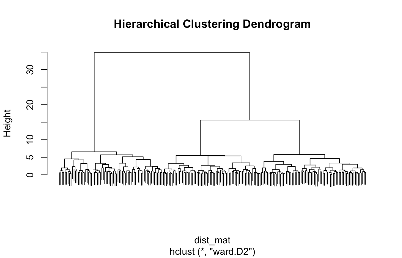
K-means provides a fast and practical way to partition observations into compact groups. Hierarchical clustering provides a nested view of structure across resolutions. Diagnostics such as elbow plots and silhouette scores help guide the analysis. Interpretation turns the output into something useful.

In both biostatistics and AI/ML, clustering is valuable because it helps transform raw heterogeneity into candidate structure.

Clustering matters because some of the most interesting patterns in data are not pre-labeled, and good analysts need tools for discovering those patterns before prediction even begins.


Tip📚 Go Deeper: Real-World Evidence Toolkit

This post is part of the Real-World Evidence Toolkit — a companion reference with patient phenotyping templates, cluster stability diagnostics, and clinical profile summary scaffolds.

→ Open the Real-World Evidence Toolkit


Series Callout

Note

This post is part of a broader Applied Statistics for AI and Clinical Decision-Making Series:

  • Probability fundamentals for machine learning
  • Random variables and expectation
  • Common probability distributions
  • Central Limit Theorem
  • Law of Large Numbers
  • Sampling methods for Biostats and ML
  • Hypothesis testing in the age of AI
  • Confidence intervals
  • Maximum likelihood estimation
  • Bayesian inference
  • Linear regression
  • Logistic regression
  • Generalized linear models
  • Analysis of variance
  • Principal component analysis
  • Cluster analysis
  • Time series analysis
  • Survival analysis
  • Non-parametric methods
  • Bias-variance tradeoff
  • Regularization
  • Cross-validation
  • Information theory
  • Optimization techniques
  • Linear algebra basics
  • Calculus for ML
  • Monte Carlo methods
  • Dimensionality curse and reduction techniques
  • Model evaluation metrics
  • Ensemble methods

References

Hastie, Trevor, Robert Tibshirani, and Jerome Friedman. 2009. The Elements of Statistical Learning: Data Mining, Inference, and Prediction. 2nd ed. Springer.
James, Gareth, Daniela Witten, Trevor Hastie, and Robert Tibshirani. 2021. An Introduction to Statistical Learning: With Applications in R. 2nd ed. Springer.
Kaufman, Leonard, and Peter J. Rousseeuw. 1990. Finding Groups in Data: An Introduction to Cluster Analysis. Wiley.
MacQueen, J. 1967. “Some Methods for Classification and Analysis of Multivariate Observations.” Proceedings of the Fifth Berkeley Symposium on Mathematical Statistics and Probability 1: 281–97.
Ward, Joe H. 1963. “Hierarchical Grouping to Optimize an Objective Function.” Journal of the American Statistical Association 58 (301): 236–44. https://doi.org/10.1080/01621459.1963.10500845.