Cross-Validation: Ensuring Your AI Isn’t Fooling Itself

Applied Statistics

AI and Clinical Decision-Making

A practical guide to K-fold cross-validation, LOOCV, stratification, and nested validation for honest model assessment in AI and applied statistics.

Published

December 15, 2024

Modified

June 9, 2026

Executive Summary

One of the easiest ways to fool yourself in modeling is to evaluate a model on the same data used to train it.

That usually leads to performance estimates that are too optimistic.

The model looks better than it really is because it is being tested on data it has already seen.

This is exactly the problem cross-validation is designed to address (Stone 1974; Arlot and Celisse 2010).

Cross-validation provides a practical way to estimate how well a model is likely to perform on new, unseen data. It does this by repeatedly splitting the data into training and validation subsets, fitting the model on one portion, and evaluating it on another.

This matters in both statistics and machine learning.

In classical modeling, cross-validation helps assess predictive performance. In AI/ML, it is one of the main tools for:

hyperparameter tuning,
model comparison,
generalization error estimation,
and guarding against overfitting.

This post introduces:

why resampling-based validation matters,
K-fold cross-validation,
leave-one-out cross-validation,
stratified sampling,
and practical implementation with R and a scikit-learn style comparison.

Cross-validation matters because good in-sample performance proves very little if the model collapses the moment it sees new data.

Cross-Validation Exists Because Training Error Is Not Enough

A model is usually optimized to fit the training data.

That means training performance is almost always biased upward as an estimate of future performance.

The more flexible the model, the more misleading training error can become.

This is why analysts distinguish between:

in-sample fit
and out-of-sample generalization

Cross-validation is one of the standard tools for estimating the second quantity.

It asks a more honest question:

how well does this model perform on data that were not used to fit it?

That is the central validation question in predictive analytics.

Generalization Error Is the Real Target

The quantity we really care about in predictive modeling is often the generalization error.

This is the expected error the model would make on future observations drawn from the same underlying process.

We cannot observe generalization error directly because we do not have access to all future data.

So we estimate it.

Cross-validation provides one practical way to do that by repeatedly holding out subsets of the observed data and treating them as pseudo-future samples.

That is why cross-validation is so central in modern model assessment.

It is not just a technical convenience. It is a way of approximating the real deployment question.

A Simple Train/Test Split Is Useful, but Limited

A basic train/test split is often the first validation strategy analysts learn.

It is simple:

fit the model on the training set
evaluate it on the test set

That is often much better than reporting training performance alone.

But it has limitations.

A single split can be unstable because results depend on exactly which observations happened to land in train versus test.

That is especially problematic when:

the dataset is small
class balance matters
or the outcome is noisy

Cross-validation improves on this by repeating the train/validation process across multiple splits.

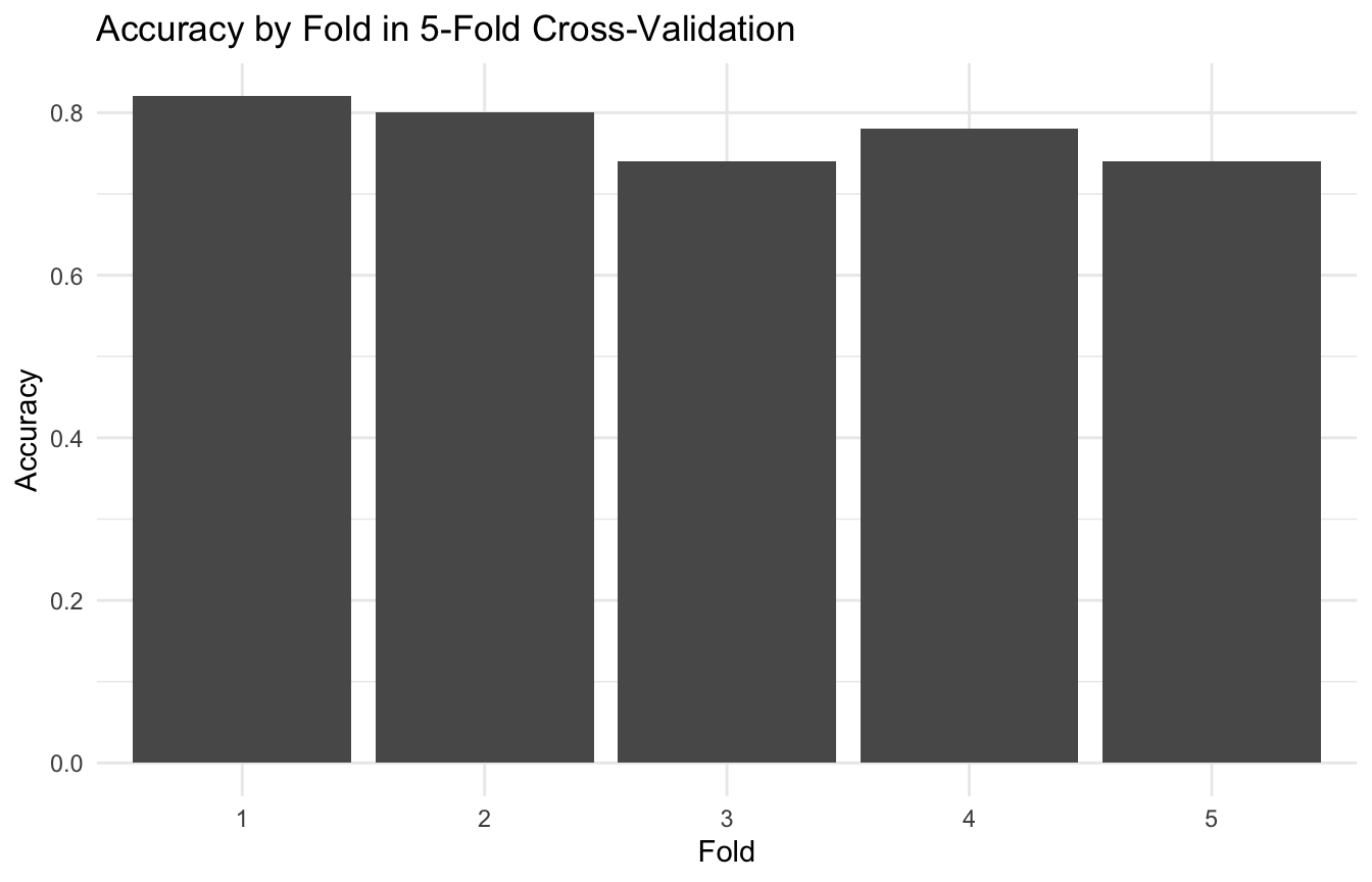
K-Fold Cross-Validation Is the Standard Workhorse

The most common version of cross-validation is K-fold cross-validation.

The data are divided into (K) roughly equal parts, or folds.

Then the model is fit (K) times:

each time using (K-1) folds for training
and the remaining fold for validation

The validation performance is averaged across all folds.

This produces a more stable estimate than a single train/test split because every observation gets a turn in the validation set.

Typical choices include:

5-fold CV
10-fold CV

These are popular because they often strike a reasonable balance between computation and stability.

A Small Example Makes the Workflow Concrete

To illustrate, we will simulate a binary classification problem with a few predictors.

library(dplyr)
library(tibble)
library(ggplot2)

n <- 250

cv_df <- tibble::tibble(
  age = rnorm(n, mean = 55, sd = 12),
  severity = rnorm(n, mean = 10, sd = 3),
  lactate = rnorm(n, mean = 2.2, sd = 0.9)
) |>
  dplyr::mutate(
    linpred = -5 + 0.04 * age + 0.30 * severity + 0.60 * lactate,
    prob = 1 / (1 + exp(-linpred)),
    event = rbinom(n, size = 1, prob = prob)
  )

cv_df |>
  dplyr::summarise(
    n = dplyr::n(),
    event_rate = mean(event)
  )

# A tibble: 1 × 2
      n event_rate
  <int>      <dbl>
1   250       0.76

This gives us a binary outcome suitable for a simple logistic regression example.

A Manual K-Fold Loop Helps Show What CV Is Actually Doing

Before using a helper package, it is often useful to see cross-validation explicitly.

Below is a simple manual 5-fold cross-validation loop using logistic regression and classification accuracy.

set.seed(20260315)

k <- 5
fold_id <- sample(rep(1:k, length.out = nrow(cv_df)))

accuracy_fun <- function(actual, predicted_prob, threshold = 0.5) {
  pred_class <- ifelse(predicted_prob >= threshold, 1, 0)
  mean(pred_class == actual)
}

cv_results <- purrr::map_dfr(
  1:k,
  function(f) {
    train_df <- cv_df[fold_id != f, ]
    valid_df <- cv_df[fold_id == f, ]
    
    fit <- glm(event ~ age + severity + lactate,
               data = train_df,
               family = binomial())
    
    valid_prob <- predict(fit, newdata = valid_df, type = "response")
    
    tibble::tibble(
      fold = f,
      accuracy = accuracy_fun(valid_df$event, valid_prob)
    )
  }
)

cv_results

# A tibble: 5 × 2
   fold accuracy
  <int>    <dbl>
1     1     0.82
2     2     0.8 
3     3     0.74
4     4     0.78
5     5     0.74

mean(cv_results$accuracy)

[1] 0.776

This code captures the main logic of K-fold CV:

split
fit
predict
evaluate
average

That is the core workflow.

K-Fold Cross-Validation Produces a Distribution, Not Just One Number

One useful feature of cross-validation is that it produces performance estimates across multiple folds.

That means we can look not only at the average performance, but also at its variability.

ggplot2::ggplot(cv_results, ggplot2::aes(x = factor(fold), y = accuracy)) +
  ggplot2::geom_col() +
  ggplot2::labs(
    title = "Accuracy by Fold in 5-Fold Cross-Validation",
    x = "Fold",
    y = "Accuracy"
  ) +
  ggplot2::theme_minimal()

This reminds us that performance is not a single magical number. It varies depending on the split.

That variability is itself informative.

Leave-One-Out Cross-Validation Uses the Data Maximally

Leave-one-out cross-validation, or LOOCV, is the extreme case of K-fold CV where:

\[ K = n \] Each model is trained on all observations except one, and then tested on that single held-out point.

This has an appealing property:

the model is fit on almost the full dataset each time

But it also has drawbacks:

it can be computationally expensive
it may have higher variance as an estimator of prediction error
it may be unnecessarily costly relative to 5-fold or 10-fold CV

Conceptually, LOOCV is useful because it shows the full logic of resampling-based validation. Practically, K-fold CV is often preferred.

A Simple LOOCV Example in R

Below is a manual LOOCV illustration.

small_df <- cv_df[1:60, ]

loocv_results <- purrr::map_dfr(
  1:nrow(small_df),
  function(i) {
    train_df <- small_df[-i, ]
    valid_df <- small_df[i, , drop = FALSE]
    
    fit <- glm(event ~ age + severity + lactate,
               data = train_df,
               family = binomial())
    
    valid_prob <- predict(fit, newdata = valid_df, type = "response")
    
    tibble::tibble(
      obs = i,
      accuracy = accuracy_fun(valid_df$event, valid_prob)
    )
  }
)

mean(loocv_results$accuracy)

[1] 0.7333333

This is computationally manageable for small examples, but becomes expensive as datasets grow.

That is one reason LOOCV is more pedagogically useful than operationally convenient in many applications.

K-Fold and LOOCV Trade Bias Against Variance and Cost

There is no universally perfect resampling scheme.

Different approaches involve tradeoffs.

LOOCV

uses almost all data for training each time
can have low bias as an error estimator
can be computationally expensive
can show higher variability

K-Fold CV

computationally more practical
often more stable in practice
widely used for tuning and model comparison

In many workflows, 5-fold or 10-fold CV is the preferred default because it performs well without excessive computation.

Stratified Sampling Matters in Classification Problems

When the outcome is binary or multiclass, especially with class imbalance, naïve random folding can create problems.

For example, one fold may contain too few positive cases, which makes evaluation unstable.

This is why stratified cross-validation is often preferred for classification.

Stratification tries to preserve the outcome proportion across folds.

That improves comparability and makes each validation fold more representative of the overall class structure.

This is especially important in biostats and clinical prediction problems where rare events matter (Harrell 2015; Steyerberg 2019).

A Simple Stratified Fold Construction in R

Below is a basic illustration of outcome-stratified fold assignment.

set.seed(20260315)

cv_df <- cv_df |>
  dplyr::group_by(event) |>
  dplyr::mutate(strat_fold = sample(rep(1:5, length.out = dplyr::n()))) |>
  dplyr::ungroup()

table(cv_df$strat_fold, cv_df$event)

This is a simple way to see the idea. Each fold contains a more balanced representation of the outcome classes.

In production workflows, this is often handled automatically by modeling libraries, but it is still important to understand the principle.

Cross-Validation Is Central to Hyperparameter Tuning

Cross-validation is not only for estimating final model performance.

It is also the standard tool for hyperparameter tuning.

Hyperparameters are choices made by the analyst rather than estimated directly by the model fit.

Examples include:

regularization strength
number of neighbors in KNN
tree depth
number of boosting iterations
penalty parameters in SVMs

Cross-validation helps choose these by asking:

which hyperparameter value performs best out of sample?

That is one of the main reasons CV is so central in ML workflows.

A Small Model-Comparison Example Makes the Point Clear

We can compare two logistic regression specifications using the same folds.

compare_cv <- purrr::map_dfr(
  1:5,
  function(f) {
    train_df <- cv_df[cv_df$strat_fold != f, ]
    valid_df <- cv_df[cv_df$strat_fold == f, ]
    
    fit_simple <- glm(event ~ age + severity,
                      data = train_df,
                      family = binomial())
    
    fit_full <- glm(event ~ age + severity + lactate,
                    data = train_df,
                    family = binomial())
    
    prob_simple <- predict(fit_simple, newdata = valid_df, type = "response")
    prob_full   <- predict(fit_full, newdata = valid_df, type = "response")
    
    tibble::tibble(
      fold = f,
      model = c("Simple", "Full"),
      accuracy = c(
        accuracy_fun(valid_df$event, prob_simple),
        accuracy_fun(valid_df$event, prob_full)
      )
    )
  }
)

compare_cv

# A tibble: 10 × 3
    fold model  accuracy
   <int> <chr>     <dbl>
 1     1 Simple     0.72
 2     1 Full       0.72
 3     2 Simple     0.7 
 4     2 Full       0.78
 5     3 Simple     0.8 
 6     3 Full       0.8 
 7     4 Simple     0.82
 8     4 Full       0.8 
 9     5 Simple     0.82
10     5 Full       0.76

And summarize the comparison.

compare_cv |>
  dplyr::group_by(model) |>
  dplyr::summarise(
    mean_accuracy = mean(accuracy),
    sd_accuracy = sd(accuracy),
    .groups = "drop"
  )

# A tibble: 2 × 3
  model  mean_accuracy sd_accuracy
  <chr>          <dbl>       <dbl>
1 Full           0.772      0.0335
2 Simple         0.772      0.0576

This is a simple example of how cross-validation supports model selection.

Cross-Validation Should Be Nested When Tuning and Evaluating

Once hyperparameters are tuned inside the same resampling loop used for performance estimation, optimism can leak back into the reported results. Nested resampling helps separate model selection from final evaluation (Hastie et al. 2009; James et al. 2021).

One common mistake is to use the same cross-validation procedure both to choose hyperparameters and to report final performance as if that were unbiased.

That can still produce overly optimistic estimates.

When hyperparameters are tuned, truly honest performance assessment often requires nested cross-validation or an external test set.

The logic is simple:

inner resampling chooses the model settings
outer resampling evaluates the tuned workflow

This distinction is important because model selection itself can overfit the resampling process.

That is one of the more subtle ways analysts fool themselves.

Cross-Validation Is Powerful, but It Is Not Magic

Cross-validation is extremely useful, but it does not fix everything.

It cannot rescue:

data leakage
poor outcome definition
nonrepresentative sampling
temporal leakage in time series
clustering dependence ignored in grouped data
or causal confounding

For example, in time series settings, ordinary random CV can be inappropriate because it breaks temporal structure.

In grouped data, subjects from the same cluster may leak information across folds.

This is why cross-validation must match the structure of the data-generating problem.

Scikit-Learn Style Thinking Maps Directly to the Same Principles

Although this post uses R, the same logic carries directly into Python and scikit-learn.

In scikit-learn, common tools include:

KFold
StratifiedKFold
cross_val_score
GridSearchCV
Pipeline

Conceptually, these do the same things:

split the data
fit models repeatedly
evaluate out-of-sample
and average results

So the statistical principle does not depend on the software language. What changes is only the implementation style.

Cross-Validation Is One of the Main Defenses Against Overfitting

In modern AI/ML, overfitting is often not obvious by inspection alone.

A highly flexible model may look impressive on the training set while performing poorly in deployment.

Cross-validation helps defend against that by forcing the model to prove itself repeatedly on held-out data.

This is why CV remains such a standard tool.

It does not guarantee that the model will succeed in the wild, but it is one of the best practical checks available before deployment.

A Practical Checklist for Applied Work

Before reporting cross-validated performance, ask:

Is the resampling strategy appropriate for the data structure?
Is stratification needed for class imbalance?
Is there any leakage across folds?
Am I tuning hyperparameters and evaluating honestly?
Would nested CV or a final test set be more appropriate?
Am I reporting only the mean, or also the variability across folds?
Would a simpler baseline perform just as well?

These questions usually improve both rigor and credibility.

Where This Shows Up in AI/ML

Temporal cross-validation — where training folds always precede validation folds in calendar time — is the required standard for clinical AI models trained on longitudinal EHR data, because random k-fold splitting allows the model to train on future data and inflate AUC by 5–15 percentage points in sepsis and deterioration prediction tasks. The Joint Pathology Center’s DoDTR-based mortality models have historically been evaluated using random splits across deployment sites, which masks the performance drop when a model trained on peacetime MTF caseloads is applied to combat casualty data with a different injury profile and care-interval distribution. When CV results from a single institution are presented as evidence of generalizability, the model has passed an exam it wrote for itself — and the failure shows up operationally, not in the development notebook.

Closing: Cross-Validation Helps Keep Models Honest

Cross-validation remains one of the most important tools in modern predictive analytics because it forces a simple but essential discipline:

do not judge a model only by how well it explains the data it already saw.

K-fold CV provides a practical and stable way to estimate generalization error (Arlot and Celisse 2010). LOOCV shows the full resampling idea in its most exhaustive form. Stratified cross-validation improves classification assessment when class balance matters. And nested approaches help keep tuning from contaminating evaluation.

Cross-validation matters because predictive performance is only meaningful if it survives contact with data the model did not get to memorize.

📚 Go Deeper: Prediction Modeling Toolkit

This post is part of the Prediction Modeling Toolkit — a companion reference with K-fold cross-validation scaffolds, stratified splitting templates, nested CV code, and hyperparameter tuning workflows.

→ Open the Prediction Modeling Toolkit

Series Callout

Note

This post is part of a broader Applied Statistics for AI and Clinical Decision-Making Series:

Probability fundamentals for machine learning
Random variables and expectation
Common probability distributions
Central Limit Theorem
Law of Large Numbers
Sampling methods for Biostats and ML
Hypothesis testing in the age of AI
Confidence intervals
Maximum likelihood estimation
Bayesian inference
Linear regression
Logistic regression
Generalized linear models
Analysis of variance
Principal component analysis
Cluster analysis
Time series analysis
Survival analysis
Non-parametric methods
Bias-variance tradeoff
Regularization
Cross-validation
Information theory
Optimization techniques
Linear algebra basics
Calculus for ML
Monte Carlo methods
Dimensionality curse and reduction techniques
Model evaluation metrics
Ensemble methods

Series: Applied Statistics for AI & Clinical Decision-Making

← Regularization Techniques: Taming Wild ML Models | Entropy in Stats: Measuring Uncertainty for Smarter AI →

References

Arlot, Sylvain, and Alain Celisse. 2010. “A Survey of Cross-Validation Procedures for Model Selection.” Statistics Surveys 4: 40–79.

Harrell, Jr., Frank E. 2015. Regression Modeling Strategies. 2nd ed. Springer.

Hastie, Trevor, Robert Tibshirani, and Jerome Friedman. 2009. The Elements of Statistical Learning: Data Mining, Inference, and Prediction. 2nd ed. Springer.

James, Gareth, Daniela Witten, Trevor Hastie, and Robert Tibshirani. 2021. An Introduction to Statistical Learning: With Applications in R. 2nd ed. Springer.

Steyerberg, Ewout W. 2019. Clinical Prediction Models: A Practical Approach to Development, Validation, and Updating. 2nd ed. Springer.

Stone, Mervyn. 1974. “Cross-Validatory Choice and Assessment of Statistical Predictions.” Journal of the Royal Statistical Society: Series B 36 (2): 111–47.