Entropy in Stats: Measuring Uncertainty for Smarter AI

Applied Statistics

AI and Clinical Decision-Making

An applied introduction to entropy, mutual information, KL divergence, and information-theoretic ideas that support modern statistics and AI.

Published

January 15, 2025

Modified

June 9, 2026

Executive Summary

Information theory gives us a formal language for uncertainty.

It asks questions like:

how uncertain is a variable?
how much information does one variable provide about another?
how inefficient is one probability model relative to another?
and how can uncertainty be encoded, compressed, or reduced?

These ideas matter deeply in both statistics and machine learning.

In classical statistics, information-theoretic ideas help quantify uncertainty and compare probability models (Shannon 1948; Cover and Thomas 2006). In AI/ML, they sit underneath:

decision tree splitting,
feature selection,
cross-entropy loss,
variational autoencoders,
and many generative modeling workflows.

This post introduces:

entropy,
conditional entropy,
mutual information,
Kullback-Leibler divergence,
and how these ideas connect to prediction, compression, and feature relevance.

Information theory matters because learning is fundamentally about reducing uncertainty, and entropy gives us a way to measure how much uncertainty is left.

Information Theory Is About Quantifying Uncertainty

At a high level, information theory gives us tools for measuring how uncertain a random variable is and how much that uncertainty changes when we observe something else.

This is useful because many statistical and ML tasks are really uncertainty problems in disguise.

For example:

a classifier tries to reduce uncertainty about a label
a feature selector asks which variable is most informative
a compressor asks how efficiently data can be encoded
a generative model asks how closely one distribution approximates another

Information theory provides a common language for all of these.

That is one reason it remains so central across fields that otherwise look quite different.

Entropy Measures Uncertainty in a Distribution

The most fundamental quantity in information theory is entropy.

For a discrete random variable (X) with probabilities (p(x)), entropy is:

\[ H(X) = -\sum_x p(x)\log p(x) \] Entropy is high when the outcome is very uncertain. Entropy is low when the outcome is predictable.

For example:

a fair coin has higher entropy than a coin that lands heads 99% of the time
a uniformly distributed categorical variable has higher entropy than one dominated by a single class

This is why entropy is often described as a measure of uncertainty, unpredictability, or information content.

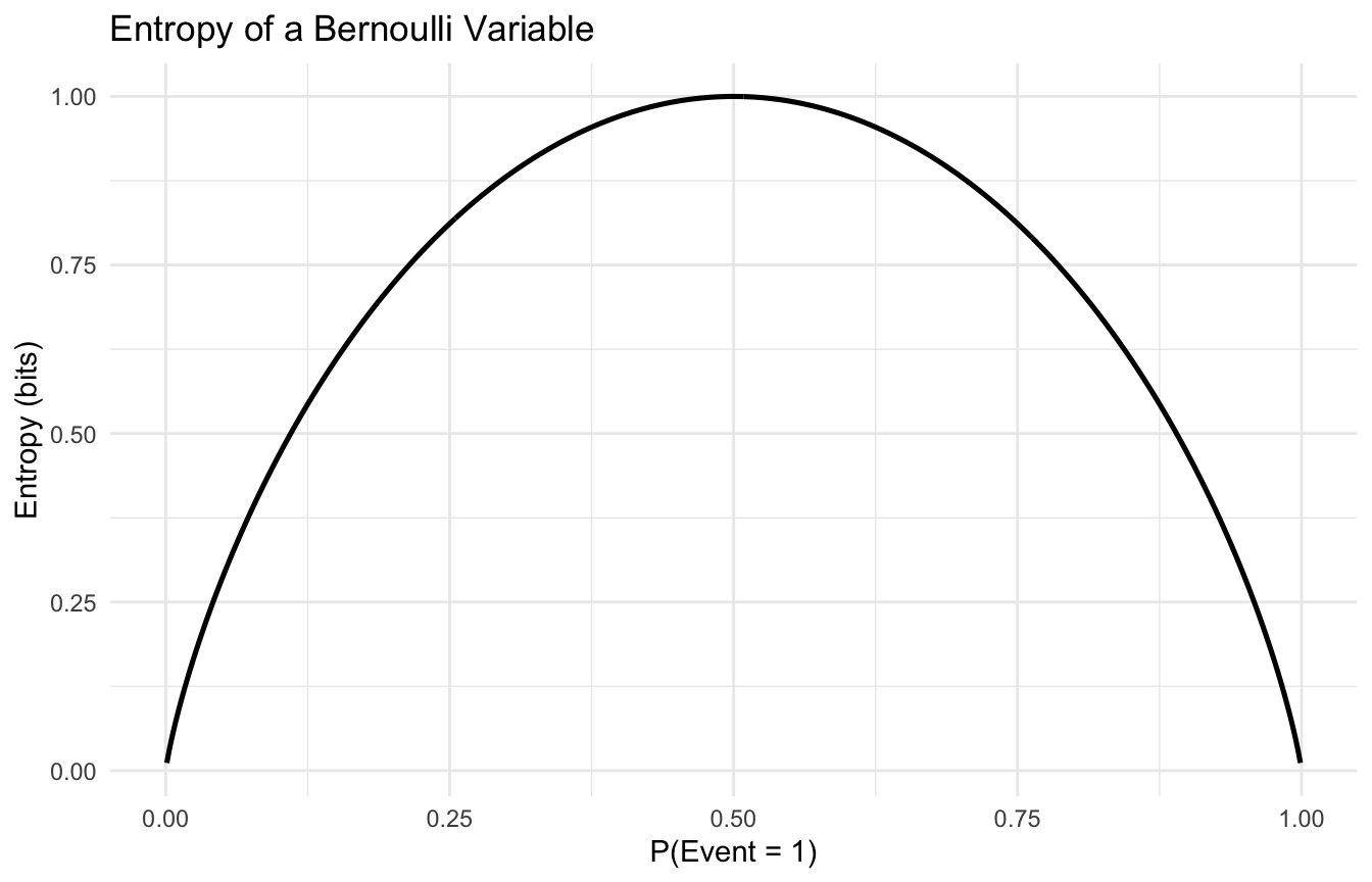
Entropy Is Highest When Outcomes Are Most Evenly Distributed

One of the most useful intuitions is that entropy is maximized when probability mass is spread evenly across possible outcomes.

If one category dominates, uncertainty is lower.

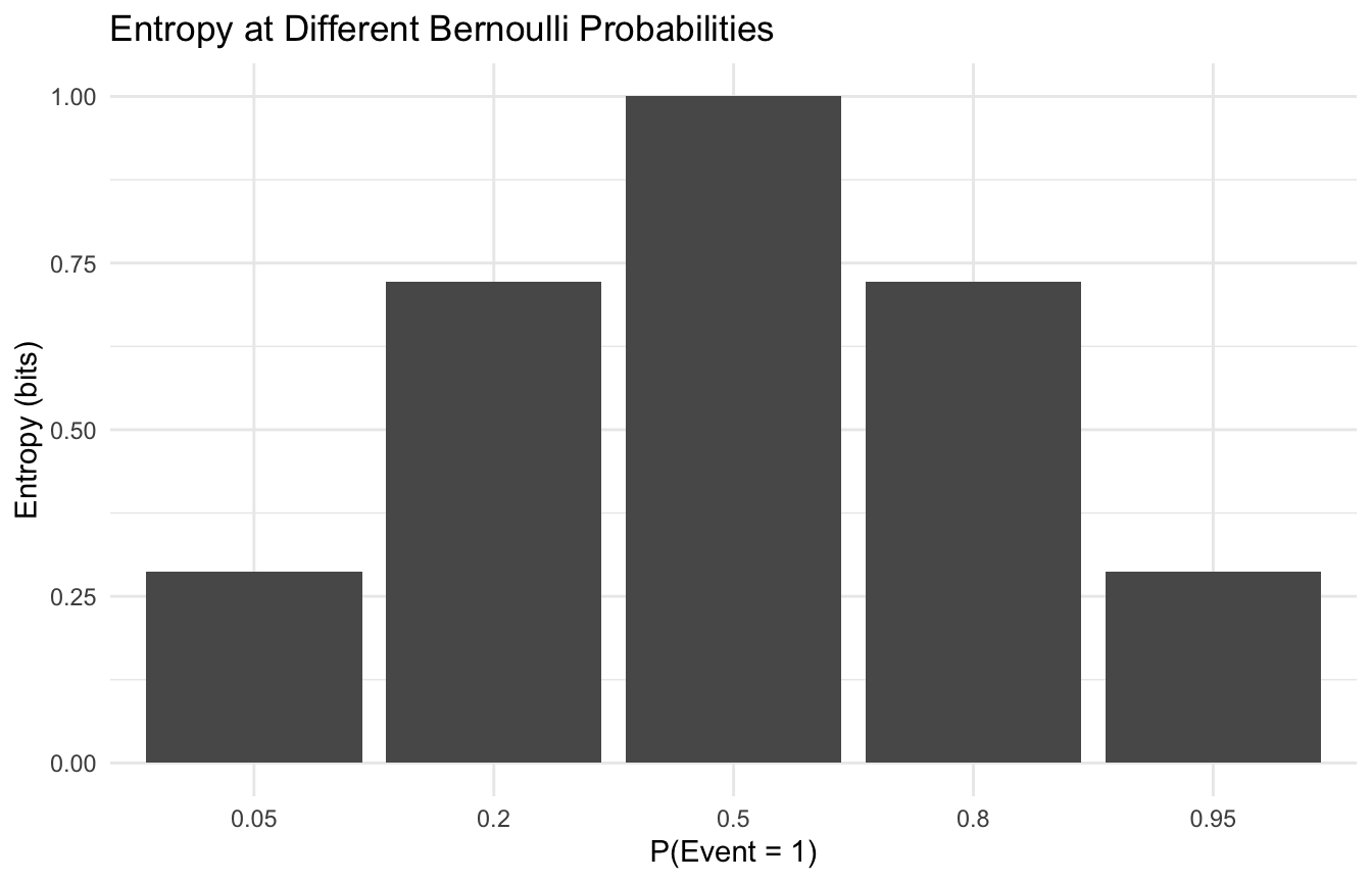
This is easy to see with a simple Bernoulli example.

library(dplyr)
library(tibble)
library(ggplot2)

entropy_bernoulli <- function(p) {
  ifelse(
    p %in% c(0, 1),
    0,
    -(p * log2(p) + (1 - p) * log2(1 - p))
  )
}

entropy_df <- tibble::tibble(
  p = seq(0.001, 0.999, length.out = 500),
  entropy = entropy_bernoulli(p)
)

ggplot2::ggplot(entropy_df, ggplot2::aes(x = p, y = entropy)) +
  ggplot2::geom_line(linewidth = 0.9) +
  ggplot2::labs(
    title = "Entropy of a Bernoulli Variable",
    x = "P(Event = 1)",
    y = "Entropy (bits)"
  ) +
  ggplot2::theme_minimal()

Entropy is highest at (p = 0.5), where the outcome is maximally uncertain.

That is one of the clearest visual ways to understand the concept.

Entropy Also Connects to Compression

One reason entropy matters beyond theory is that it is closely linked to data compression.

If an outcome is highly predictable, it can be encoded more efficiently. If it is highly uncertain, it takes more bits on average to represent.

That means entropy is not only a measure of uncertainty. It is also a lower-bound style guide to how efficiently data can be compressed.

This is one reason the idea became so important historically in communications and coding theory.

It is also why entropy is such a natural bridge between statistics and computer science.

In AI/ML, this compression perspective reappears in latent representations, coding efficiency, and model-based summarization.

A Small Categorical Example Makes Entropy Concrete

Suppose we observe a variable representing triage category, phenotype group, or clinical class label.

We can compute its empirical entropy directly from observed frequencies.

cat_df <- tibble::tibble(
  class = c("A", "A", "A", "A", "B", "B", "C", "C", "C", "D")
)

class_probs <- cat_df |>
  dplyr::count(class) |>
  dplyr::mutate(
    p = n / sum(n)
  )

class_probs

# A tibble: 4 × 3
  class     n     p
  <chr> <int> <dbl>
1 A         4   0.4
2 B         2   0.2
3 C         3   0.3
4 D         1   0.1

Now compute entropy.

emp_entropy <- -sum(class_probs$p * log2(class_probs$p))
emp_entropy

[1] 1.846439

This gives the uncertainty of the observed class distribution in bits.

That number is a summary of how unpredictable the class label is before we observe any predictor.

Conditional Entropy Measures Remaining Uncertainty

Entropy tells us how uncertain a variable is on its own.

But often the more interesting question is:

how uncertain is the outcome after we observe another variable?

That is the idea of conditional entropy:

\[ H(Y \mid X) \] This measures how much uncertainty remains in (Y) once (X) is known.

If knowing (X) makes (Y) nearly predictable, then the conditional entropy is low. If knowing (X) changes very little, then the conditional entropy remains high.

This quantity is central to feature usefulness.

A good predictor reduces uncertainty about the target.

Mutual Information Measures How Informative One Variable Is About Another

A key information-theoretic quantity for applied work is mutual information.

Mutual information between (X) and (Y) is:

\[ I(X;Y) = H(Y) - H(Y \mid X) \] It can also be written symmetrically as:

\[ I(X;Y) = H(X) + H(Y) - H(X,Y) \] This tells us how much knowing one variable reduces uncertainty about the other.

Properties:

it is always nonnegative
it equals zero if the variables are independent
larger values mean stronger information-sharing

This makes mutual information especially useful for feature selection and exploratory variable ranking.

A Feature Selection Example with Mutual Information

Suppose we have a binary outcome and two candidate predictors.

One predictor is informative. The other is mostly noise.

We can simulate that idea.

n <- 300

mi_df <- tibble::tibble(
  informative_feature = sample(c("Low", "High"), size = n, replace = TRUE),
  noisy_feature = sample(c("A", "B"), size = n, replace = TRUE)
) |>
  dplyr::mutate(
    event = dplyr::if_else(
      informative_feature == "High",
      rbinom(n, size = 1, prob = 0.75),
      rbinom(n, size = 1, prob = 0.30)
    )
  )

We can define a small helper to compute entropy and mutual information for discrete variables.

entropy_discrete <- function(x) {
  probs <- table(x) / length(x)
  probs <- probs[probs > 0]
  -sum(probs * log2(probs))
}

joint_entropy_discrete <- function(x, y) {
  probs <- table(x, y) / length(x)
  probs <- probs[probs > 0]
  -sum(probs * log2(probs))
}

mutual_information_discrete <- function(x, y) {
  entropy_discrete(x) + entropy_discrete(y) - joint_entropy_discrete(x, y)
}

Now compute mutual information between each feature and the outcome.

mi_tbl <- tibble::tibble(
  feature = c("informative_feature", "noisy_feature"),
  mutual_information = c(
    mutual_information_discrete(mi_df$informative_feature, mi_df$event),
    mutual_information_discrete(mi_df$noisy_feature, mi_df$event)
  )
)

mi_tbl

# A tibble: 2 × 2
  feature             mutual_information
  <chr>                            <dbl>
1 informative_feature           0.210   
2 noisy_feature                 0.000133

The informative feature should show higher mutual information because it reduces uncertainty about the event more strongly.

Mutual Information Can Detect Nonlinear Dependence Better Than Correlation

One of the reasons mutual information is so useful is that it is not limited to linear association.

Correlation is excellent for linear relationships, but it can miss nonlinear dependence.

Mutual information is more general. If two variables share information, mutual information can detect that even when the relationship is not linear in a simple correlation sense.

That is one reason information-theoretic feature selection is often attractive in machine learning pipelines.

It can sometimes identify useful predictors that a purely linear screening approach might understate.

Decision Trees Use Entropy to Split Data

One of the clearest machine learning applications of entropy is in decision trees.

In tree algorithms like ID3, the goal is to split the data so that child nodes are more homogeneous in the target than the parent node (Cover and Thomas 2006; Hastie et al. 2009).

This is measured through information gain:

\[ \text{Information Gain} = H(Y) - H(Y \mid X) \] That is exactly mutual information between the splitting feature and the target.

So when a tree selects a split that maximally reduces entropy, it is directly applying an information-theoretic criterion.

This is one of the reasons information theory matters so much in ML: the ideas are not abstract decorations. They actively shape model construction.

KL Divergence Measures How Different Two Distributions Are

Kullback-Leibler divergence formalizes the information lost when one probability distribution is used to approximate another (Kullback and Leibler 1951).

Another major quantity in information theory is Kullback-Leibler divergence, or KL divergence.

For two discrete distributions (P) and (Q):

\[ D_{KL}(P \parallel Q) = \sum_x P(x)\log\left(\frac{P(x)}{Q(x)}\right) \] KL divergence is often interpreted as a measure of how inefficient it is to use distribution (Q) to approximate data actually generated from (P).

Important cautions:

it is not symmetric
it is not a true distance metric
it is always nonnegative when well-defined

But it is extremely useful for comparing probabilistic models.

A Small KL Divergence Example Makes the Idea Concrete

Suppose the true outcome distribution is:

(P = (0.7, 0.2, 0.1))

and a model approximates it with:

(Q = (0.5, 0.3, 0.2))

We can compute KL divergence directly.

P <- c(0.7, 0.2, 0.1)
Q <- c(0.5, 0.3, 0.2)

kl_div <- sum(P * log2(P / Q))
kl_div

[1] 0.1228063

If (Q) matched (P) exactly, the KL divergence would be zero.

The farther (Q) departs from (P), the larger the divergence tends to become.

This is why KL divergence is widely used in model comparison, variational inference, and generative modeling.

Cross-Entropy and KL Divergence Show Up in ML Loss Functions

Many machine learning practitioners encounter information theory through cross-entropy loss.

Cross-entropy is closely related to entropy and KL divergence.

In classification, minimizing cross-entropy encourages the predicted distribution to align closely with the true label distribution.

In broader terms:

entropy measures intrinsic uncertainty
cross-entropy measures coding cost under an approximating model
KL divergence measures the excess inefficiency of one distribution relative to another

These ideas appear directly in:

logistic regression loss
neural network classification
generative models
and variational autoencoders

This is one reason information theory is not a side topic. It is embedded in the loss functions that drive modern learning systems.

Entropy Also Helps Explain Why Compression and Representation Matter

A useful way to connect information theory to modern AI is through representation.

Many ML systems try to learn compressed representations that retain signal while discarding redundancy.

This is a kind of information management problem.

Good representations:

reduce irrelevant variation
preserve predictive structure
and make the downstream task easier

That is one reason entropy-based thinking fits so naturally with:

latent variable models
autoencoders
compression-inspired learning
and uncertainty-aware modeling

The underlying question is often the same:

how much uncertainty remains, and how efficiently can useful information be represented?

A Visual Entropy Comparison Can Help Build Intuition

Below is a simple comparison of entropy across several Bernoulli probabilities.

entropy_bar_df <- tibble::tibble(
  p = c(0.05, 0.20, 0.50, 0.80, 0.95),
  entropy = entropy_bernoulli(p)
)

ggplot2::ggplot(entropy_bar_df, ggplot2::aes(x = factor(p), y = entropy)) +
  ggplot2::geom_col() +
  ggplot2::labs(
    title = "Entropy at Different Bernoulli Probabilities",
    x = "P(Event = 1)",
    y = "Entropy (bits)"
  ) +
  ggplot2::theme_minimal()

This helps reinforce that uncertainty is highest near balanced probabilities and lower near near-certain outcomes.

Information-Theoretic Feature Selection Is Useful, but Not Sufficient Alone

Mutual information can be a powerful feature-screening tool, but it should not be treated as the whole modeling story.

A feature may have:

low marginal mutual information but strong joint value with other features
high mutual information but unstable measurement
or strong association that is operationally irrelevant

So information-theoretic ranking is often useful for:

screening
exploration
and variable prioritization

But it should still be embedded within a broader modeling and validation strategy.

This is especially important in high-dimensional applied work.

Information Theory Connects Statistics, ML, and Computation

One reason information theory is so powerful is that it naturally links several domains.

It speaks simultaneously to:

probability distributions
uncertainty
coding and compression
feature relevance
predictive loss
and model mismatch

This makes it one of the most conceptually unifying topics in modern analytics.

A statistician may encounter entropy through uncertainty. A machine learning practitioner may encounter it through cross-entropy loss. A computer scientist may encounter it through compression.

The underlying logic is the same.

A Practical Checklist for Applied Work

Before using information-theoretic tools, ask:

Am I measuring uncertainty, dependence, or model mismatch?
Is entropy the right summary for the problem?
Is mutual information being estimated in a way appropriate to the variable type?
Would correlation miss important nonlinear structure here?
Is KL divergence being interpreted as a directional comparison, not a distance?
Am I using information-theoretic screening as a first step rather than the only step?
Does the ML loss function I am using have an information-theoretic meaning worth understanding?

These questions usually improve both interpretation and application.

Where This Shows Up in AI/ML

Every neural network trained for clinical prediction — sepsis onset, deterioration, 30-day readmission — minimizes cross-entropy loss during training, which is the direct information-theoretic measure of how far the model’s predicted probability distribution is from the true label distribution. KL divergence is used in production ML monitoring pipelines to detect distribution shift: when the KL divergence between the feature distribution at training time and the feature distribution at inference time exceeds a threshold, the model is flagged for recalibration — a process directly applicable to DoDTR-based models redeployed across different operational theaters. When cross-entropy is replaced with a surrogate loss without understanding its information-theoretic meaning, or when KL-based drift detection is skipped, models silently degrade against populations they were never shown.

Closing: Information Theory Gives Analytics a Language for Uncertainty

Information theory remains one of the most important conceptual bridges in modern analytics because it gives us a way to measure uncertainty, relevance, and model mismatch with precision.

Entropy quantifies unpredictability. Mutual information tells us how much uncertainty one variable removes from another. KL divergence measures how costly it is to approximate one distribution with another.

These are not merely elegant formulas (Cover and Thomas 2006). They are active ingredients in feature selection, decision trees, generative modeling, compression, and modern AI loss functions.

Information theory matters because learning is, at its core, the process of turning uncertainty into structure, and entropy tells us how much uncertainty we started with.

📚 Go Deeper: Prediction Modeling Toolkit

This post is part of the Prediction Modeling Toolkit — a companion reference with entropy-based feature selection templates, mutual information code, and cross-entropy loss scaffolds for classification models.

→ Open the Prediction Modeling Toolkit

Series Callout

Note

This post is part of a broader Applied Statistics for AI and Clinical Decision-Making Series:

Probability fundamentals for machine learning
Random variables and expectation
Common probability distributions
Central Limit Theorem
Law of Large Numbers
Sampling methods for Biostats and ML
Hypothesis testing in the age of AI
Confidence intervals
Maximum likelihood estimation
Bayesian inference
Linear regression
Logistic regression
Generalized linear models
Analysis of variance
Principal component analysis
Cluster analysis
Time series analysis
Survival analysis
Non-parametric methods
Bias-variance tradeoff
Regularization
Cross-validation
Information theory
Optimization techniques
Linear algebra basics
Calculus for ML
Monte Carlo methods
Dimensionality curse and reduction techniques
Model evaluation metrics
Ensemble methods

Series: Applied Statistics for AI & Clinical Decision-Making

← Cross-Validation: Ensuring Your AI Isn’t Fooling Itself | Optimization Essentials: The Engine of Modern AI →

References

Cover, Thomas M., and Joy A. Thomas. 2006. Elements of Information Theory. 2nd ed. Wiley-Interscience.

Hastie, Trevor, Robert Tibshirani, and Jerome Friedman. 2009. The Elements of Statistical Learning: Data Mining, Inference, and Prediction. 2nd ed. Springer.

Kullback, Solomon, and Richard A. Leibler. 1951. On Information and Sufficiency. 22 (1): 79–86.

Shannon, Claude E. 1948. “A Mathematical Theory of Communication.” Bell System Technical Journal 27 (3): 379–423.