A practical introduction to gradients, gradient descent, SGD, mini-batch updates, and learning-rate ideas that power modern AI model training.
Published
February 15, 2025
Modified
June 9, 2026
Executive Summary
Modern machine learning models do not usually solve themselves.
They are trained.
That training process is, at its core, an optimization problem.
A model begins with unknown parameters. A loss function tells us how poorly the model is performing. An optimizer updates the parameters to reduce that loss.
Gradient-based optimization is one of the most important ideas in machine learning because it provides a general mechanism for fitting models when closed-form solutions are unavailable or impractical.
These methods matter because they power:
linear and logistic regression fitting under some formulations,
neural network training,
deep learning optimization,
regularized objective functions,
and many modern large-scale predictive systems.
This post introduces:
gradients,
batch gradient descent,
stochastic gradient descent,
mini-batch updates,
learning rates,
and why these ideas remain central even when more advanced optimizers such as Adam are used.
Optimization matters because even the best model architecture is useless if its parameters cannot be trained toward a better solution.
Optimization Is the Hidden Engine of Model Training
Many modeling workflows present the final fitted model as if it simply appears after a function call.
But underneath that function call is often an optimization problem.
At a high level, model training asks:
what parameter values minimize the loss?
how should we move through parameter space?
how fast should those updates happen?
and how do we avoid getting stuck or diverging?
These questions are not only computational. They shape whether a model learns well at all.
This is why optimization is not a side topic in AI/ML. It is the engine of training.
A Loss Function Gives the Model Something to Improve
Optimization requires an objective.
In supervised learning, that objective is often a loss function.
Examples include:
mean squared error for regression
log loss for classification
negative log-likelihood for probabilistic models
The model is trained by choosing parameters that reduce this loss.
That means optimization is never floating in the abstract. It is always tied to a specific objective.
So before asking how gradient descent works, it helps to ask:
what exactly is being minimized?
That is the quantity the optimizer is trying to improve.
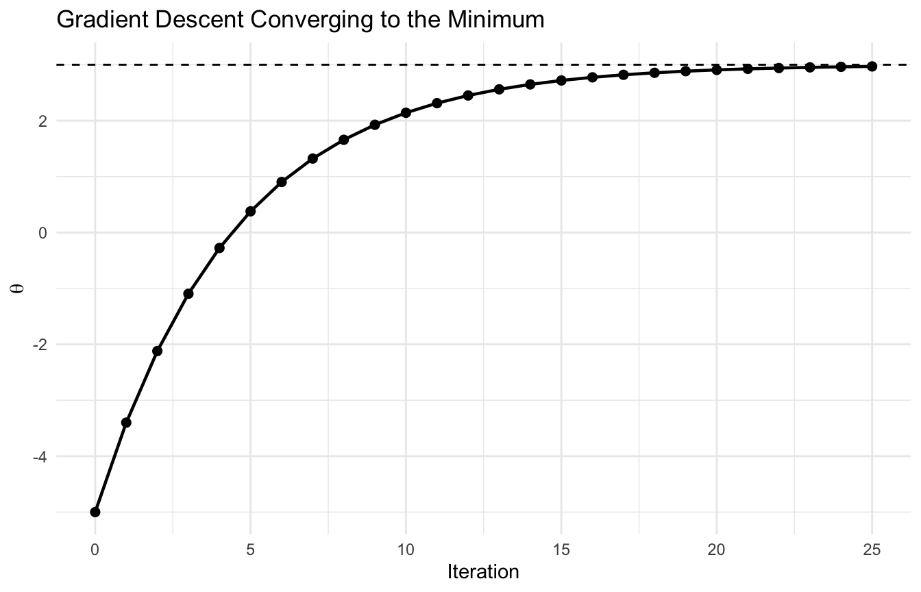
The Gradient Points in the Direction of Steepest Increase
The key mathematical object in gradient-based optimization is the gradient.
For a function of one variable, the derivative tells us the slope.
For a function of multiple parameters, the gradient collects the partial derivatives:
\[
\nabla L(\theta) =
\left(
\frac{\partial L}{\partial \theta_1},
\frac{\partial L}{\partial \theta_2},
\dots,
\frac{\partial L}{\partial \theta_p}
\right)
\] This vector points in the direction of steepest increase of the loss.
If we want to minimize the loss, we should move in the opposite direction.
This shows the parameter moving toward the optimal value iteratively.
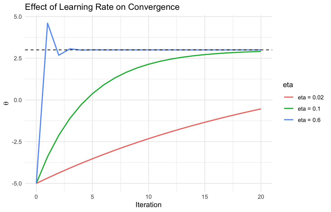
The Learning Rate Controls How Aggressive the Updates Are
The learning rate, often written (), is one of the most important tuning parameters in gradient-based optimization.
It controls the size of each update step.
If the learning rate is too small:
learning can be painfully slow
If the learning rate is too large:
updates may overshoot the minimum
the algorithm may oscillate
or it may diverge entirely
This is why learning rate choice can strongly affect whether training succeeds.
We can compare several learning rates.
run_gd <-function(theta_init, eta, n_steps =20) { theta <- theta_init out <- tibble::tibble(step =0, theta = theta, eta =paste0("eta = ", eta))for (i in1:n_steps) { theta <- theta - eta *grad_fn(theta) out <- dplyr::bind_rows( out, tibble::tibble(step = i, theta = theta, eta =paste0("eta = ", eta)) ) } out}eta_df <- dplyr::bind_rows(run_gd(theta_init =-5, eta =0.02),run_gd(theta_init =-5, eta =0.10),run_gd(theta_init =-5, eta =0.60))ggplot2::ggplot(eta_df, ggplot2::aes(x = step, y = theta, color = eta)) + ggplot2::geom_line(linewidth =0.8) + ggplot2::geom_hline(yintercept =3, linetype =2) + ggplot2::labs(title ="Effect of Learning Rate on Convergence",x ="Iteration",y =expression(theta) ) + ggplot2::theme_minimal()
This is one of the clearest ways to show why optimization is sensitive to tuning.
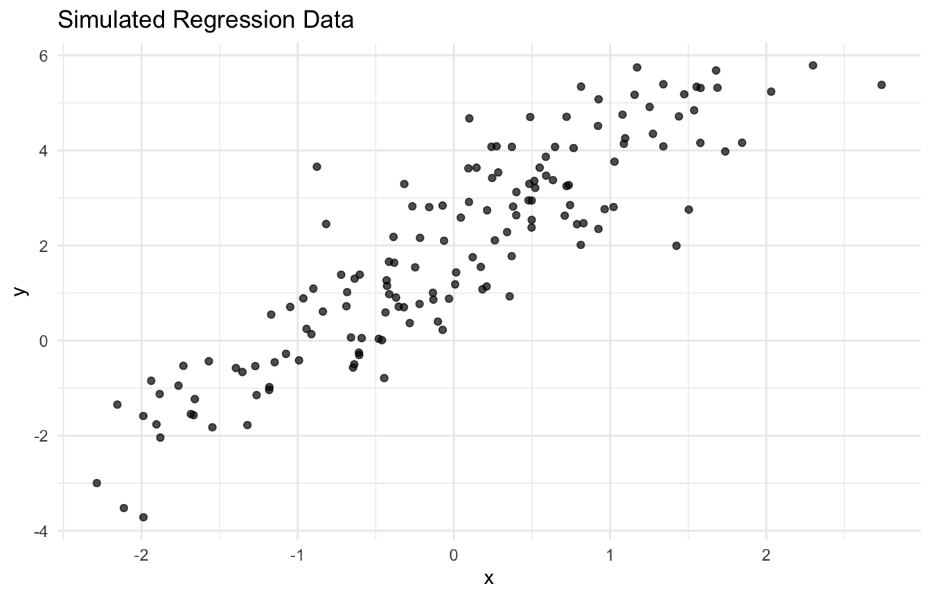
Gradient Descent Can Be Applied to Linear Regression
A familiar loss function is the regression mean squared error:
\[
L(\beta_0, \beta_1) = \frac{1}{n} \sum_{i=1}^n (y_i - (\beta_0 + \beta_1 x_i))^2
\] Although linear regression has a closed-form solution under ordinary least squares, it is still useful to fit it with gradient descent as a teaching device.
This shows how iterative optimization works in a real model.
n <-150opt_df <- tibble::tibble(x =rnorm(n, mean =0, sd =1)) |> dplyr::mutate(y =2+1.8* x +rnorm(n, mean =0, sd =1) )ggplot2::ggplot(opt_df, ggplot2::aes(x = x, y = y)) + ggplot2::geom_point(alpha =0.7) + ggplot2::theme_minimal() + ggplot2::labs(title ="Simulated Regression Data",x ="x",y ="y" )
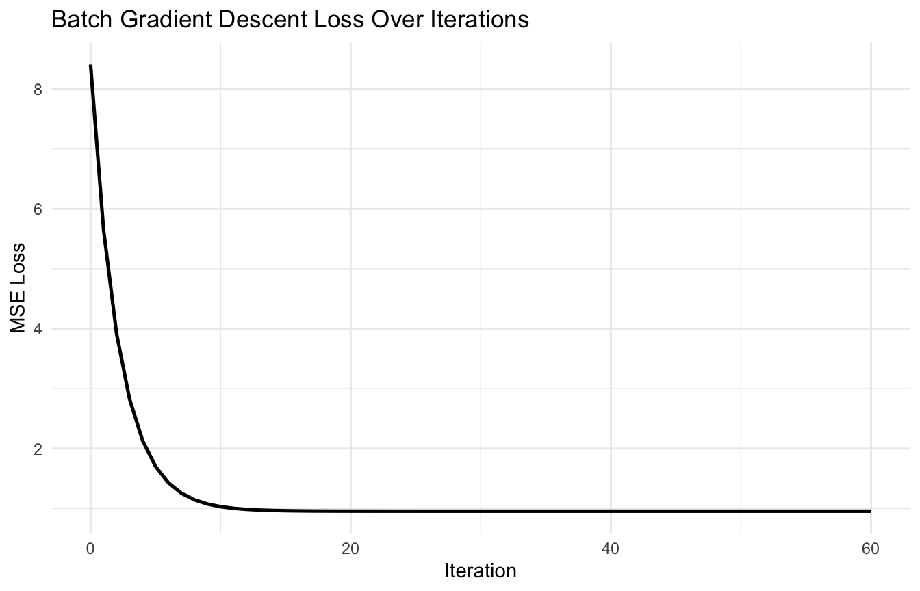
ggplot2::ggplot(reg_path, ggplot2::aes(x = step, y = loss)) + ggplot2::geom_line(linewidth =0.9) + ggplot2::labs(title ="Batch Gradient Descent Loss Over Iterations",x ="Iteration",y ="MSE Loss" ) + ggplot2::theme_minimal()
This shows the optimizer progressively reducing the loss.
Batch Gradient Descent Uses the Full Dataset Each Update
The version above is batch gradient descent.
At each iteration, it computes the gradient using the full dataset.
Advantages:
stable updates
exact gradient for the current parameters
conceptually simple
Disadvantages:
computationally expensive for large datasets
can be slow when data are massive
This is one reason machine learning moved toward stochastic and mini-batch variants for large-scale problems.
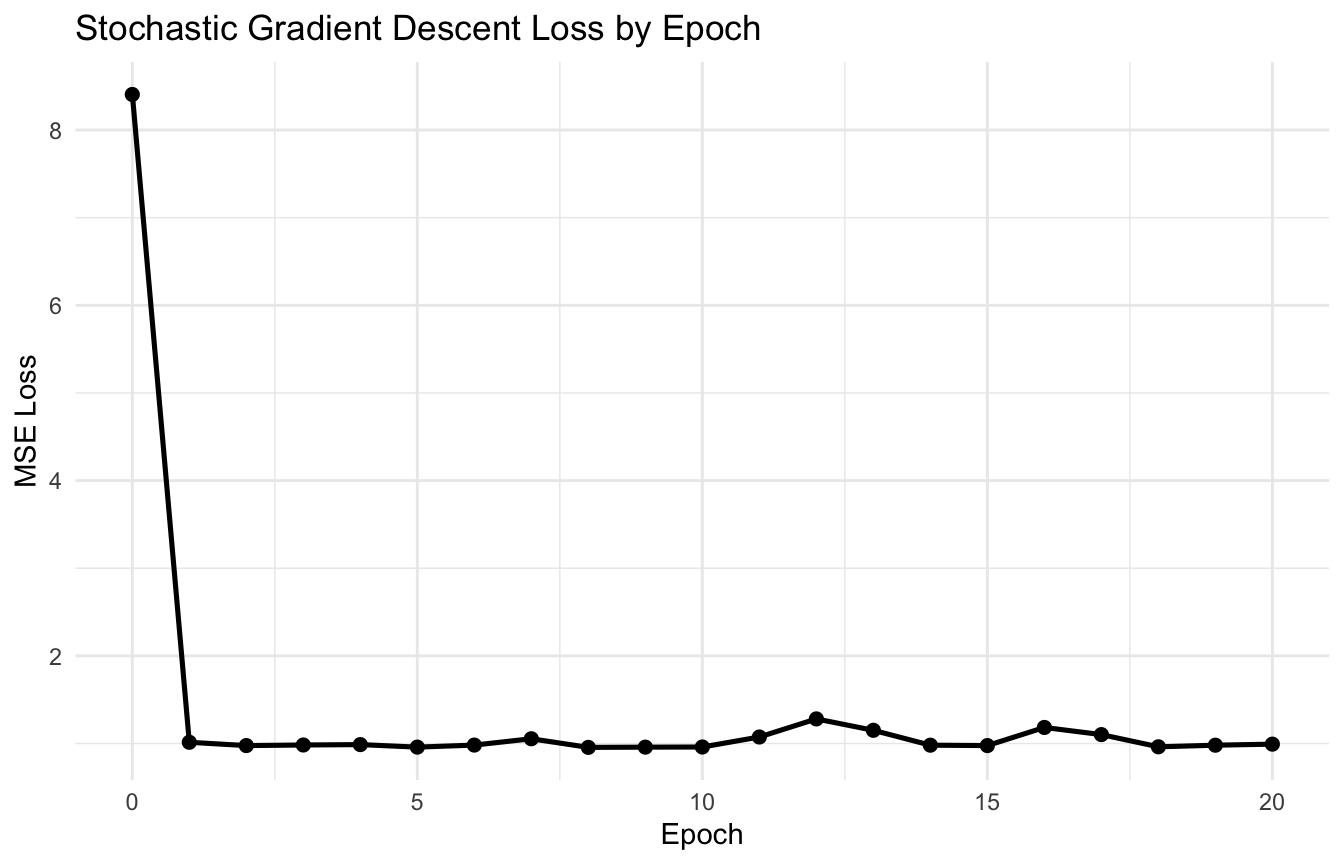
Stochastic Gradient Descent Uses One Observation at a Time
The stochastic approximation idea underlying SGD goes back to Robbins and Monro and remains one of the core conceptual bridges from classical optimization to modern large-scale learning (Robbins and Monro 1951).
Stochastic gradient descent, or SGD, updates the parameters using just one observation at a time.
Instead of computing a full gradient over all (n) points, SGD uses a noisy estimate of the gradient from a single case.
This makes updates:
much cheaper
noisier
often faster in wall-clock terms
and capable of escaping some optimization traps
Conceptually, SGD trades precision in the update for computational speed.
That tradeoff is one of the reasons it became so important in large-scale learning.
A Simple SGD Example Shows the Noisier Path
We can implement SGD for the same regression problem.
b0 <-0b1 <-0eta <-0.05n_epochs <-20sgd_path <- tibble::tibble(epoch =0,b0 = b0,b1 = b1,loss =mse_loss(b0, b1, opt_df$x, opt_df$y))for (epoch in1:n_epochs) { idx <-sample(seq_len(nrow(opt_df)))for (i in idx) { xi <- opt_df$x[i] yi <- opt_df$y[i] pred_i <- b0 + b1 * xi err_i <- yi - pred_i b0 <- b0 - eta * (-2* err_i) b1 <- b1 - eta * (-2* xi * err_i) } sgd_path <- dplyr::bind_rows( sgd_path, tibble::tibble(epoch = epoch,b0 = b0,b1 = b1,loss =mse_loss(b0, b1, opt_df$x, opt_df$y) ) )}sgd_path
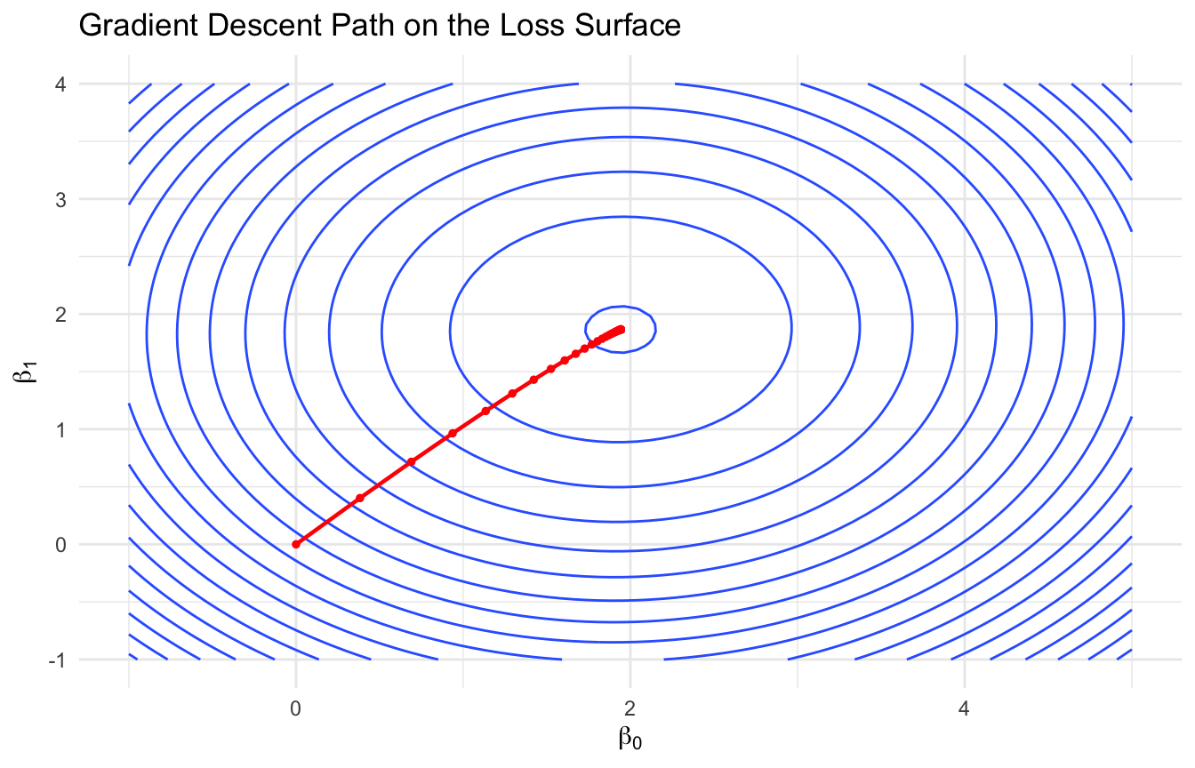
ggplot2::ggplot(surface_df, ggplot2::aes(x = b0, y = b1, z = loss)) + ggplot2::geom_contour(bins =20) + ggplot2::geom_path(data = reg_path, ggplot2::aes(x = b0, y = b1),color ="red",linewidth =0.8 ) + ggplot2::geom_point(data = reg_path, ggplot2::aes(x = b0, y = b1),color ="red",size =1 ) + ggplot2::labs(title ="Gradient Descent Path on the Loss Surface",x =expression(beta[0]),y =expression(beta[1]) ) + ggplot2::theme_minimal()
This is one of the most intuitive ways to show what optimization is doing geometrically.
Optimization Problems Can Be Harder Than This Toy Example
The examples so far are friendly.
Real optimization can be much messier.
Challenges include:
non-convex loss surfaces
saddle points
flat regions
exploding gradients
vanishing gradients
noisy updates
badly scaled features
This is why optimization in deep learning is not just “run gradient descent and wait.” It often requires thoughtful tuning, normalization, and algorithm choice (Goodfellow et al. 2016).
Still, the basic gradient idea remains the foundation.
Feature Scaling Often Helps Gradient-Based Optimization
A very practical lesson is that optimization behaves better when predictors are on comparable scales.
If one feature has a much larger scale than another, the loss surface can become stretched and poorly conditioned.
This makes optimization slower and less stable.
That is why standardization is often helpful before gradient-based training.
Feature scaling does not change the conceptual model, but it can dramatically improve how efficiently the optimizer moves through parameter space.
This is especially important in:
linear models fit iteratively
neural networks
regularized optimization
and distance-sensitive ML methods
SGD Is the Bridge to Modern Deep Learning
Why is SGD so central in AI/ML?
Because modern models can involve:
millions of parameters
huge training datasets
and objectives that cannot be solved analytically
In those settings, batch-style exact optimization is often too slow.
SGD and mini-batch methods make training feasible.
That is why these techniques are not just classroom algorithms. They are the operational core of large-scale model training.
Neural networks, in particular, depend heavily on stochastic optimization.
Advanced Optimizers Extend the Same Core Logic
Methods such as Adam retain the same update logic while adapting step sizes using running moments of the gradients (Kingma and Ba 2015).
Modern optimizers such as:
Momentum
RMSProp
Adam
do not replace gradient descent conceptually. They extend it.
These methods still use gradients, but they add mechanisms such as:
adaptive step sizes
momentum accumulation
running averages of gradient information
This can improve convergence, especially in large, noisy, or poorly conditioned problems.
But the foundation remains the same:
compute gradients
update parameters
reduce the loss
That is why understanding plain gradient descent is still essential.
Optimization Is Not Just a Technical Detail
One of the biggest mistakes in applied ML is to treat optimization as if it were only a software implementation detail.
It is not.
Optimization affects:
whether the model converges
how stable the estimates are
how long training takes
and whether the final fitted solution is actually useful
This is especially important when comparing model architectures.
Sometimes a “better” model fails in practice because its training dynamics are poor. Sometimes a simpler model succeeds because it is easier to optimize reliably.
That is why optimization deserves conceptual attention, not only code execution.
A Practical Checklist for Applied Work
Before training a gradient-based model, ask:
What loss function is being optimized?
Are the gradients available analytically or through automatic differentiation?
Is the learning rate appropriate?
Should training use batch, stochastic, or mini-batch updates?
Are the features scaled appropriately?
Is the loss decreasing in a stable way?
Would a learning rate schedule help?
Is a more advanced optimizer such as Adam warranted?
These questions often matter as much as the model architecture itself.
NoteWhere This Shows Up in AI/ML
The Adam optimizer — a gradient descent variant using adaptive per-parameter learning rates — is the default training algorithm for virtually every clinical NLP model applied to trauma documentation, including ICD code prediction from free-text operative notes and injury severity extraction from TCCC cards. When the learning rate is set too high during fine-tuning of a pretrained model on a small trauma registry dataset, the optimizer overshoots the loss minimum and produces erratic weight updates that can destroy the pretrained representations rather than refine them — a failure mode called catastrophic forgetting. Clinicians seeing a model that performed well in development perform erratically in deployment often cannot trace the problem to optimizer misconfiguration, but that is frequently what happened upstream.
Closing: Optimization Turns Models into Trained Systems
Optimization remains one of the most important ideas in modern AI because it is what turns a model specification into a trained system.
Gradient descent provides the core logic. SGD and mini-batch methods make large-scale learning practical. Learning rates determine how updates behave. Advanced optimizers extend the same principles to more difficult training settings.
This is why optimization is not merely background machinery. It is a central part of how modern models actually learn.
Optimization matters because building a model is only the beginning, and training it well is what makes the model useful.
This post is part of the Prediction Modeling Toolkit — a companion reference with gradient descent implementation templates, learning rate selection guidance, and loss surface diagnostic scaffolds.