v <- c(2, 4, 6)
w <- c(1, -1, 3)

v
[1] 2 4 6w[1] 1 -1 3Linear algebra is one of the quiet foundations of modern statistics and machine learning.
It sits underneath:
For many applied analysts, linear algebra can feel more abstract than probability or regression (Strang 2016; Golub and Van Loan 2013). But in practice, it is often the language that makes those methods possible.
Vectors represent observations, features, parameters, and gradients. Matrices represent datasets, transformations, covariance structures, and systems of equations. Eigenvalues and eigenvectors reveal dominant directions of variation. Singular value decomposition provides a closely related factorization that is foundational for PCA, compression, and latent representation (Eckart and Young 1936; Jolliffe 2002). Singular value decomposition powers dimension reduction and latent representation.
This post introduces:
Linear algebra matters because modern statistical and AI models do not only analyze numbers, they transform whole data structures.
A dataset is not just a collection of variables. It is often best thought of as a matrix.
In applied work:
This is why linear algebra matters so much (Strang 2016).
It gives us a compact and powerful way to express:
Once the data are written in matrix form, many statistical procedures become much easier to state and compute.
A vector is an ordered collection of numbers.
In statistics and ML, vectors are everywhere.
Examples include:
A vector can represent either:
depending on the context.
In R, vectors are easy to create.
v <- c(2, 4, 6)
w <- c(1, -1, 3)
v[1] 2 4 6w[1] 1 -1 3Basic vector operations include addition, subtraction, and scalar multiplication.
v + w[1] 3 3 9v - w[1] 1 5 32 * v[1] 4 8 12These simple operations become building blocks for more complex model computations.
One of the most important vector operations is the dot product.
For vectors (v) and (w),
\[ v^\top w = \sum_i v_i w_i \] This operation appears constantly in modeling.
For example, a linear predictor in regression can be written as a dot product between:
sum(v * w)[1] 16This is not just algebraic convenience. It is the core computational form behind many predictive models.
A single prediction in a linear model is essentially a weighted sum, which is naturally expressed as a dot product.
A matrix is a rectangular array of numbers.
In applied statistics, a matrix can represent:
Here is a simple example.
A <- matrix(
  c(1, 2,
    3, 4,
    5, 6),
  nrow = 3,
  byrow = TRUE
)

A
[,1] [,2]
[1,] 1 2
[2,] 3 4
[3,] 5 6This is a (3 ) matrix.
Its dimensions matter because matrix operations depend on shape compatibility.
dim(A)[1] 3 2nrow(A)[1] 3ncol(A)[1] 2Matrices are not just storage objects. They encode relationships among values in structured form.
Matrix multiplication is one of the most important operations in all of statistics and ML.
If (A) is an (n p) matrix and (b) is a (p ) vector, then (Ab) produces an (n ) vector.
This is exactly the structure of linear prediction.
X <- matrix(
  c(1, 2,
    1, 3,
    1, 4),
  nrow = 3,
  byrow = TRUE
)

beta <- matrix(c(0.5, 2), ncol = 1)

X
[,1] [,2]
[1,] 1 2
[2,] 1 3
[3,] 1 4beta [,1]
[1,] 0.5
[2,] 2.0X %*% beta [,1]
[1,] 4.5
[2,] 6.5
[3,] 8.5Here:
X can be thought of as a design matrix,beta as a coefficient vector,X %*% beta as the predicted values.This is one reason matrix multiplication is so central. It turns a whole set of observations into predictions at once.
The transpose of a matrix flips rows and columns.
If (X) is an (n p) matrix, then (X^) is a (p n) matrix.
In R, transpose is computed with t().
X [,1] [,2]
[1,] 1 2
[2,] 1 3
[3,] 1 4t(X) [,1] [,2] [,3]
[1,] 1 1 1
[2,] 2 3 4Transpose operations are essential because many formulas in statistics depend on them.
For example:
all use transposes extensively.
Many statistical problems reduce to solving systems of linear equations.
For example, ordinary least squares regression can be written in matrix form as:
\[ \hat{\beta} = (X^\top X)^{-1} X^\top y \] That formula itself is a linear algebra statement.
Before going to regression, consider a simpler system:
\[ Ax = b \] where:
A2 <- matrix(c(2, 1,
               1, 3), nrow = 2, byrow = TRUE)

b2 <- c(5, 7)

solve(A2, b2)
[1] 1.6 1.8This is the computational idea behind many estimation procedures: find the unknown vector that satisfies a matrix equation.
A matrix inverse is often written as (A^{-1}), but not every matrix has one.
A matrix must be square and nonsingular to be invertible.
In R, the inverse can be computed with solve(A) when it exists.
solve(A2) [,1] [,2]
[1,] 0.6 -0.2
[2,] -0.2 0.4In practice, applied analysts often rely on matrix decompositions rather than explicitly computing inverses whenever possible, especially in larger or less stable systems.
That is because direct inversion can be numerically fragile.
So while the inverse is important conceptually, modern computation often prefers more stable matrix factorizations.
One of the most important matrix objects in statistics is the covariance matrix.
For a multivariable dataset, the covariance matrix summarizes:
This makes it a compact description of how variables vary jointly.
Let us simulate a small multivariable dataset.
cov_df <- tibble::tibble(
  x1 = rnorm(200, mean = 0, sd = 1),
  x2 = 0.7 * x1 + rnorm(200, mean = 0, sd = 0.7),
  x3 = -0.4 * x1 + 0.5 * x2 + rnorm(200, mean = 0, sd = 0.8)
)

cov_mat <- cov(cov_df)
cov_mat
x1 x2 x3
x1 1.054799254 0.7799018 -0.007899273
x2 0.779901768 1.0084821 0.201021132
x3 -0.007899273 0.2010211 0.761381436This matrix is a key input for many multivariate procedures.
The covariance matrix is important because it tells us more than separate variances.
It reveals how variables move together.
That matters in:
A visual can help.
cov_long <- as.data.frame(as.table(cov_mat)) |>
  tibble::as_tibble() |>
  dplyr::rename(
    Var1 = Var1,
    Var2 = Var2,
    Covariance = Freq
  )

ggplot2::ggplot(cov_long, ggplot2::aes(x = Var1, y = Var2, fill = Covariance)) +
  ggplot2::geom_tile() +
  ggplot2::labs(
    title = "Covariance Matrix Heatmap",
    x = NULL,
    y = NULL
  ) +
  ggplot2::theme_minimal()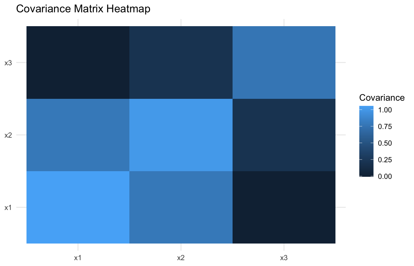
This helps make the joint structure more visible than the raw matrix printout alone.
A major reason covariance matrices matter is that we can decompose them into eigenvalues and eigenvectors.
If (A) is a square matrix, an eigenvector (v) satisfies:
\[ Av = \lambda v \] where () is the corresponding eigenvalue.
Interpretation:
This is one of the key ideas behind PCA.
In covariance analysis:
We can compute the eigen decomposition of the covariance matrix directly.
eig <- eigen(cov_mat)

eig$values
[1] 1.8290207 0.7857518 0.2098902eig$vectors [,1] [,2] [,3]
[1,] 0.7033442 -0.2762189 0.6549886
[2,] 0.6995028 0.1049652 -0.7068792
[3,] 0.1265024 0.9553457 0.2670425The eigenvalues tell us the amount of variance captured by each principal direction.
The eigenvectors tell us how those directions are constructed from the original variables.
This is exactly why linear algebra is so central to dimension reduction.
In PCA, the covariance matrix or correlation matrix is decomposed into eigenvalues and eigenvectors.
This means PCA is not just a statistical trick. It is a linear algebra operation with a strong statistical interpretation.
In practice:
This is one reason PCA is such a natural bridge between statistics and machine learning. It is both algebraic and data-analytic at once.
A broader and extremely important decomposition is the singular value decomposition, or SVD (Eckart and Young 1936; Strang 2016).
If (X) is a data matrix, then:
\[ X = UDV^\top \] where:
SVD is powerful because it works for rectangular matrices, not only square ones.
This makes it central to:
SVD is one of the most important decompositions in applied linear algebra.
We can apply SVD directly to a centered data matrix.
X_centered <- scale(cov_df, center = TRUE, scale = FALSE)

svd_fit <- svd(X_centered)

svd_fit$d
[1] 19.078132 12.504584 6.462829svd_fit$u[1:5, ] [,1] [,2] [,3]
[1,] -0.07112137 -0.05583428 -0.08088451
[2,] 0.03713521 0.06178893 0.01738438
[3,] -0.03422936 0.01020568 -0.05705661
[4,] 0.05426623 0.03649346 -0.05474664
[5,] 0.12455487 0.02908866 -0.01942323svd_fit$v [,1] [,2] [,3]
[1,] -0.7033442 -0.2762189 0.6549886
[2,] -0.6995028 0.1049652 -0.7068792
[3,] -0.1265024 0.9553457 0.2670425The singular values summarize the strength of the dominant directions. The singular vectors define the corresponding structure in row and column space.
In PCA, these singular values are closely related to the variances explained by the principal components.
One reason SVD matters so much is that it supports low-rank approximation.
Instead of keeping the full matrix, we can approximate it using only the largest singular values and their associated vectors.
This is useful because it allows us to:
That is exactly the logic behind many dimension-reduction workflows.
It is also why matrix factorization methods became so important in recommendation systems and latent representation learning.
In recommendation systems, analysts often work with large user-item matrices.
These matrices are:
Matrix factorization methods use linear algebra to decompose these large matrices into lower-dimensional latent factors.
This lets the system learn things like:
So the same ideas that appear in covariance decomposition and PCA also appear in recommender systems and embeddings.
That is why linear algebra is not just a prerequisite topic. It is active machinery in modern AI.
Even neural networks, which may look conceptually far removed from classical multivariate analysis, depend fundamentally on linear algebra.
Each layer in a neural network typically involves:
That means forward propagation itself is largely a sequence of structured linear algebra operations.
The deeper model adds more layers and nonlinearities, but the computational engine still depends on vectors, matrices, and transformations.
So linear algebra remains central even in models that appear highly modern or highly nonlinear.
A useful way to summarize the linear algebra story in statistics is:
This workflow connects directly to:
That is why the covariance matrix example is so valuable. It shows how statistics and linear algebra meet in a concrete way.
Before using linear algebra tools in modeling, ask:
These questions usually improve both understanding and implementation.
The transformer attention mechanism inside every modern clinical NLP model — including those used to extract injury descriptors from trauma narratives and discharge summaries — is a set of matrix multiplications that compute weighted relationships between token embeddings; there is no architectural component that is not a linear algebraic operation. When a trauma NLP model is applied to documentation that uses abbreviations or terminology outside its training vocabulary, the token embeddings for those inputs land in regions of the vector space that were poorly covered during training, producing confidently wrong extractions. SVD underlies the latent semantic analysis pipelines used to cluster similar injury narratives in OMOP-structured trauma registries, and a poorly conditioned input matrix — from sparse or duplicated records — will produce singular values that amplify noise rather than structure.
Linear algebra remains essential because it provides the structure and operations that let modern statistics and machine learning scale beyond isolated formulas.
Vectors represent features and parameters. Matrices represent data and transformations. Covariance matrices summarize joint variation. Eigenvalues and eigenvectors reveal dominant structure. SVD supports compression, factorization, and modern representation learning.
Linear algebra matters because once data become multivariable, analysis becomes less about single numbers and more about structured transformations.
This post is part of the Prediction Modeling Toolkit — a companion reference with matrix operation templates, covariance matrix diagnostics, SVD decomposition code, and linear algebra scaffolds for clinical modeling.
This post is part of a broader Applied Statistics for AI and Clinical Decision-Making Series: