Calculus Crash Course: Derivatives Driving AI Innovation
Applied Statistics
AI and Clinical Decision-Making
An applied introduction to derivatives, gradients, the chain rule, and integrals for understanding optimization and backpropagation in AI.
Published
April 15, 2025
Modified
June 9, 2026
Executive Summary
Calculus is one of the quiet engines of machine learning.
It explains how models learn, how loss functions change, and how tiny parameter updates become large-scale improvements in prediction (Stewart 2015; Goodfellow et al. 2016).
For many analysts, calculus can feel more abstract than regression, hypothesis testing, or even linear algebra. But in modern AI/ML, it is everywhere.
Derivatives tell us:
how sensitive a loss function is to a parameter,
how steeply an objective is changing,
and which direction reduces error fastest.
Partial derivatives extend this idea to many-parameter models. The chain rule makes backpropagation possible, and that chain-rule logic is exactly what modern backpropagation algorithms exploit in deep learning (Rumelhart et al. 1986; Goodfellow et al. 2016). Integrals connect continuously varying uncertainty to quantities like expectation and probability (Stewart 2015; Murphy 2012).
This post introduces:
derivatives,
partial derivatives,
the chain rule,
basic integrals,
and why these ideas matter for gradient-based learning.
Calculus matters because training a model is really the problem of understanding how small changes in parameters change the loss.
Calculus Is the Language of Change
At a high level, calculus is about change.
It gives us tools for asking:
how fast is a quantity changing?
how sensitive is one variable to another?
how much total quantity accumulates over a range?
and how do small local changes build into a global result?
These questions are central in machine learning.
A model is trained by changing parameters. A loss function measures the consequences of those changes. An optimizer uses derivatives to decide how to update the model (Goodfellow et al. 2016; Boyd and Vandenberghe 2004).
That is why calculus is not peripheral to ML. It is one of the main mathematical languages of learning.
Derivatives Measure Local Sensitivity
The derivative of a function tells us how rapidly the function changes as its input changes.
If we have a function (f(x)), then the derivative (f’(x)) measures the slope at a point.
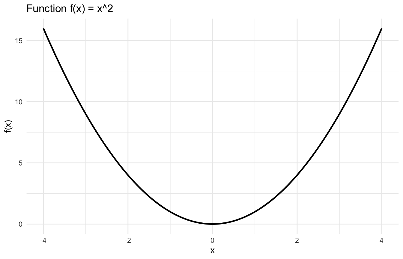
For example, if:
\[
f(x) = x^2
\]
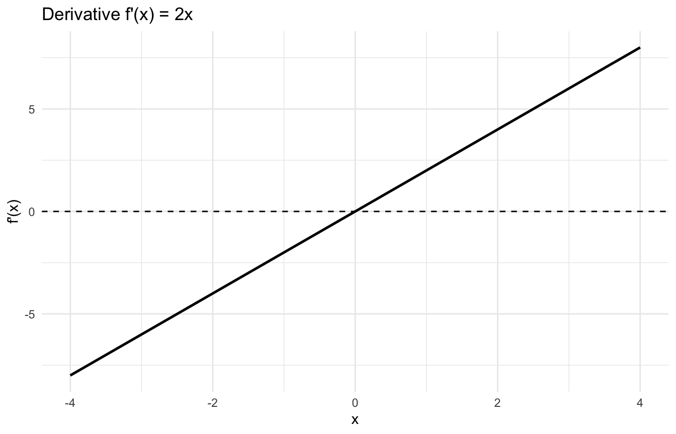
then:
\[
f'(x) = 2x
\]
This means:
when (x) is large and positive, the function is increasing steeply,
when (x) is near zero, the slope is shallow,
and when (x) is negative, the slope is negative.
In machine learning, this is exactly the kind of information we need. The derivative tells us how a loss function responds to a parameter change.
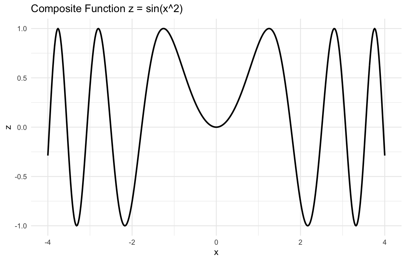
A Simple Derivative Example Makes the Idea Concrete
Let us define a simple function and its derivative.
This makes the derivative visible as a slope function rather than only a symbolic object.
Derivatives Are Central to Loss Minimization
A loss function tells us how poorly a model is performing.
To improve the model, we need to know how the loss changes as the parameters change.
That is exactly what derivatives provide.
If the derivative is positive, increasing the parameter may increase the loss. If the derivative is negative, increasing the parameter may reduce the loss. If the derivative is near zero, the model may be near a minimum or a flat region.
This is why optimization methods like gradient descent depend on derivatives. They use slope information to decide which direction reduces the loss.
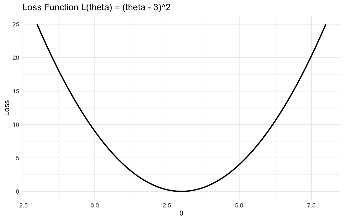
A Quadratic Loss Example Shows Why Derivatives Matter
Suppose the loss is:
\[
L(\theta) = (\theta - 3)^2
\]
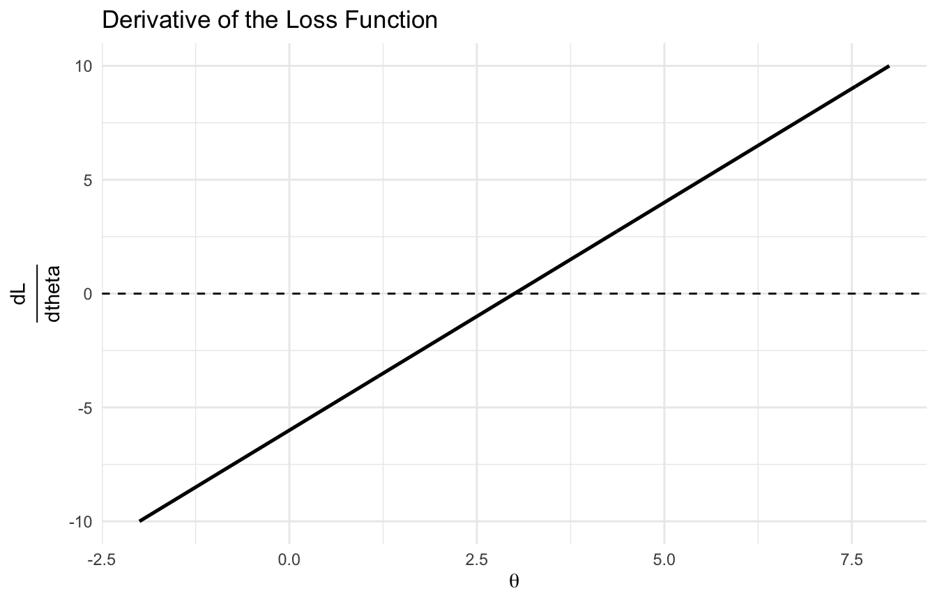
Then:
\[
\frac{dL}{d\theta} = 2(\theta - 3)
\]
This derivative tells us:
if (> 3), the slope is positive, so moving left reduces the loss
if (< 3), the slope is negative, so moving right reduces the loss
if (= 3), the slope is zero, so the loss is minimized
This is a small example, but the same logic scales to very large layered models.
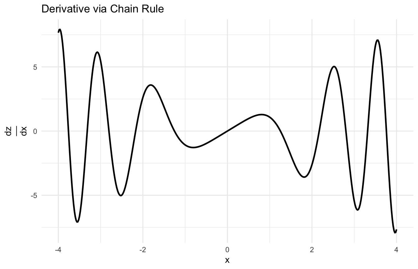
Backpropagation Is Repeated Chain Rule
Neural networks are built from many nested transformations.
At a high level, a network might compute:
a linear combination,
then an activation,
then another linear combination,
then another activation,
and finally a loss.
To train the network, we need the derivative of the loss with respect to each weight.
That derivative is not computed independently from scratch for each parameter. Instead, backpropagation works backward through the network, repeatedly applying the chain rule.
This is why the chain rule is not merely a calculus exercise. It is one of the central mathematical ideas behind deep learning.
Integrals Represent Accumulation
So far, calculus has appeared through derivatives and gradients. But integrals matter too.
An integral represents accumulation.
For a function (f(x)), the integral over an interval measures total accumulated quantity:
\[
\int_a^b f(x),dx
\]
In probability and statistics, integrals are often used for:
total probability,
expectation,
marginalization,
and continuous distributions.
This is why integrals remain important for ML too, especially in probabilistic modeling.
Expectations in Continuous Models Are Often Integrals
For a continuous random variable (X) with density (f(x)), the expectation of a function (g(X)) is:
\[
E[g(X)] = \int g(x) f(x),dx
\]
That means integration is part of how we compute:
expected value,
variance,
likelihood-based summaries,
and many Bayesian quantities.
A simple example is the expected value of a standard normal variable, which is 0 by symmetry.
While many applied analysts rely on software rather than hand integration, the conceptual role of the integral remains important.
It is the continuous analog of weighted summation.
A Simple Numerical Integration Example Helps Ground the Idea
Suppose we want to numerically integrate a density-like function.
This returns approximately 1, as expected for a density.
Now a simple expectation-like calculation.
g_expectation <-function(x) x *dnorm(x, mean =0, sd =1)integrate(g_expectation, lower =-Inf, upper =Inf)
0 with absolute error < 0
This is approximately 0, as expected.
These examples help connect integration to probability rather than treating it as only geometric area.
Calculus Connects Loss, Learning, and Uncertainty
One of the most useful ways to understand calculus in ML is to see how its major ideas connect.
Derivatives tell us:
how the loss changes locally
Partial derivatives tell us:
how each parameter affects the loss
The chain rule tells us:
how layered transformations pass influence backward
Integrals tell us:
how uncertainty accumulates and is summarized in continuous models
These are not separate topics. They are different pieces of the same mathematical framework for learning from data.
Calculus Is Not Only for Neural Networks
It is easy to associate calculus mainly with deep learning, but it matters far more broadly.
Calculus appears in:
optimization of regression losses
maximum likelihood estimation
Bayesian posterior computation
survival likelihoods
gradient-based regularized models
time series parameter estimation
and probabilistic expectations
That is why calculus belongs in the foundation of ML, not only in advanced neural-network discussions.
It is part of the language of model fitting itself.
Loss Minimization Is One of the Most Important Applied Uses of Calculus
A major theme in machine learning is loss minimization.
Once a loss function is defined, the next question is how to move the model parameters in a direction that reduces it.
That is a calculus question.
Without derivatives, the optimizer has no local information about:
slope
curvature
or parameter sensitivity
This is why derivatives drive so many training algorithms.
Even when modern software computes them automatically, understanding their role is still important for interpreting how training works.
Automatic Differentiation Does Not Replace Understanding
Modern ML frameworks often use automatic differentiation to compute gradients efficiently.
This is incredibly useful in practice.
But it does not make the calculus irrelevant.
Instead, it makes calculus operational at scale.
The software is still using:
derivatives
partial derivatives
and chain rule logic
So even if analysts no longer compute every derivative by hand, understanding the underlying ideas remains valuable.
It helps explain:
why gradients behave as they do
why learning rates matter
and why some models train better than others
A Practical Checklist for Applied Work
Before using calculus-driven optimization in a model, ask:
What loss function is being minimized?
Which parameters does the loss depend on?
Are the gradients interpretable and stable?
Does the model involve layered compositions that require chain-rule reasoning?
Are gradients being computed analytically, numerically, or automatically?
Is the optimization sensitive to scaling or learning rate?
Are integrals or expectations part of the modeling problem?
These questions often make model training much easier to understand.
NoteWhere This Shows Up in AI/ML
Backpropagation — the algorithm that trains every deep clinical AI model, from retinal screening classifiers to sepsis prediction networks — is a direct implementation of the chain rule applied layer by layer from the loss function back through the network weights. In deep networks trained on small trauma datasets, vanishing gradients are a concrete failure mode: the chain rule multiplications across many layers drive the early-layer gradients toward zero, those weights stop updating, and the model effectively ignores lower-level feature representations — producing a model that is deep in name only. When clinicians ask why a mortality prediction model trained on DoDTR data performs worse on patients with polytrauma than on isolated TBI, part of the answer is often gradient flow: the compound injury signal is harder to propagate back through a network that was not designed to handle it.
Closing: Calculus Gives Machine Learning Its Sense of Direction
Calculus remains one of the most important mathematical foundations of AI and machine learning because it tells models how to improve.
Derivatives measure local change. Partial derivatives extend that logic to many-parameter systems. The chain rule makes layered learning possible. Integrals connect continuous uncertainty to expectation and probability.
Together, these ideas make it possible to define, analyze, and optimize learning systems.
Calculus matters because machine learning is not only about building models, but about understanding how to move those models toward lower error and better predictions.
This post is part of the Prediction Modeling Toolkit — a companion reference with gradient computation templates, backpropagation intuition, and numerical differentiation scaffolds for applied model training.
Boyd, Stephen, and Lieven Vandenberghe. 2004. Convex Optimization. Cambridge University Press.
Goodfellow, Ian, Yoshua Bengio, and Aaron Courville. 2016. Deep Learning. MIT Press.
Murphy, Kevin P. 2012. Machine Learning: A Probabilistic Perspective. MIT Press.
Rumelhart, David E., Geoffrey E. Hinton, and Ronald J. Williams. 1986. “Learning Representations by Back-Propagating Errors.”Nature 323 (6088): 533–36. https://doi.org/10.1038/323533a0.