Monte Carlo Magic: Simulating Uncertainty in AI

Applied Statistics
AI and Clinical Decision-Making
A practical introduction to Monte Carlo integration, importance sampling, and MCMC for uncertainty quantification, Bayesian inference, and AI.
Published

May 15, 2025

Modified

June 9, 2026

Executive Summary

Some of the most important questions in statistics and machine learning do not have neat closed-form answers.

For example:

  • what is the expected loss under a complicated posterior?
  • what is the uncertainty around a treatment effect in a hierarchical model?
  • how likely is a rare but high-cost event?
  • how do we approximate an integral in high dimensions when exact calculation is impossible?

This is where Monte Carlo methods become essential.

Monte Carlo methods use random sampling to approximate quantities that are difficult to compute analytically (Robert and Casella 2004; Owen 2013). They are especially useful for:

  • integration,
  • uncertainty quantification,
  • Bayesian inference,
  • risk simulation,
  • and high-dimensional probabilistic modeling.

This post introduces:

  • the basic Monte Carlo idea,
  • importance sampling,
  • Markov chain Monte Carlo,
  • Metropolis-Hastings,
  • and why these methods matter for simulation-based inference in both biostatistics and AI/ML (Metropolis et al. 1953; Hastings 1970).

Monte Carlo methods matter because when exact mathematics becomes intractable, carefully designed randomness can still give us useful answers.


Monte Carlo Methods Turn Random Sampling into Approximation

The central idea of Monte Carlo methods is simple:

if we can sample from the right distribution, we can approximate difficult quantities by averaging over those samples.

This is powerful because many important statistical quantities are expectations or integrals (Robert and Casella 2004; Owen 2013).

For example:

  • posterior means,
  • tail probabilities,
  • predictive uncertainty,
  • expected utility,
  • or risk measures

can often be written as integrals.

When those integrals are hard to solve analytically, simulation provides a practical alternative.

That is one reason Monte Carlo methods sit at the intersection of probability, computation, and applied inference.


Monte Carlo Integration Is Often Just Averaging

Suppose we want to compute:

\[ E[g(X)] \]

for some random variable (X).

If we can draw samples (X_1, X_2, , X_n) from the distribution of (X), then we can approximate the expectation with:

\[ \frac{1}{n}\sum_{i=1}^n g(X_i) \]

This is the core Monte Carlo idea.

It is conceptually simple, but extremely general.

Instead of solving the integral directly, we replace it with an empirical average over simulated draws.

That move is one of the main reasons simulation became so central to modern statistics and ML.


A Simple Monte Carlo Example Makes the Idea Concrete

Suppose (X N(0,1)), and we want to approximate:

\[ E[X^2] \]

We know analytically that this equals 1, but we can estimate it through simulation.

library(dplyr)
library(tibble)
library(ggplot2)

n_sims <- 10000

mc_df <- tibble::tibble(
  x = rnorm(n_sims, mean = 0, sd = 1),
  g_x = x^2
)

mc_df |>
  dplyr::summarise(
    monte_carlo_estimate = mean(g_x)
  )
# A tibble: 1 × 1
  monte_carlo_estimate
                 <dbl>
1                 1.00

The estimate should be close to 1.

This is a simple example, but it captures the main logic: simulate, transform, average.


Monte Carlo Accuracy Improves with More Draws

Monte Carlo estimates are random because they depend on the simulated sample.

But as the number of draws increases, the estimate typically becomes more stable.

We can visualize the running estimate.

mc_running_df <- mc_df |>
  dplyr::mutate(
    iter = dplyr::row_number(),
    running_est = cumsum(g_x) / iter
  )

ggplot2::ggplot(mc_running_df, ggplot2::aes(x = iter, y = running_est)) +
  ggplot2::geom_line(linewidth = 0.8) +
  ggplot2::geom_hline(yintercept = 1, linetype = 2) +
  ggplot2::labs(
    title = "Running Monte Carlo Estimate of E[X^2]",
    x = "Simulation Draw",
    y = "Estimate"
  ) +
  ggplot2::theme_minimal()

This reinforces a key idea:

  • Monte Carlo does not produce exact answers instantly,
  • but with enough draws, it often produces useful approximations.

Importance Sampling Reweights Samples from a Convenient Distribution

Basic Monte Carlo works well when we can sample directly from the target distribution.

But sometimes that is difficult.

This is where importance sampling becomes useful.

Suppose we want an expectation under a target distribution (p(x)), but it is easier to sample from another distribution (q(x)).

Then we can reweight the draws:

$$ E_p[g(X)] = g(x)p(x),dx ================

g(x)q(x),dx $$

This leads to the importance sampling estimator:

\[ \frac{1}{n}\sum_{i=1}^n g(X_i)\frac{p(X_i)}{q(X_i)} \]

where the (X_i) are sampled from (q).

The weights correct for the fact that we sampled from the wrong distribution.


A Small Importance Sampling Example Shows the Logic

Suppose we want to estimate the mean of a standard normal target distribution using draws from a wider normal proposal.

This is not necessary here, but it illustrates the method.

n_sims <- 10000

x_prop <- rnorm(n_sims, mean = 0, sd = 2)

target_density <- dnorm(x_prop, mean = 0, sd = 1)
proposal_density <- dnorm(x_prop, mean = 0, sd = 2)

weights <- target_density / proposal_density

is_estimate <- sum(x_prop * weights) / sum(weights)

tibble::tibble(
  importance_sampling_estimate = is_estimate
)
# A tibble: 1 × 1
  importance_sampling_estimate
                         <dbl>
1                      0.00371

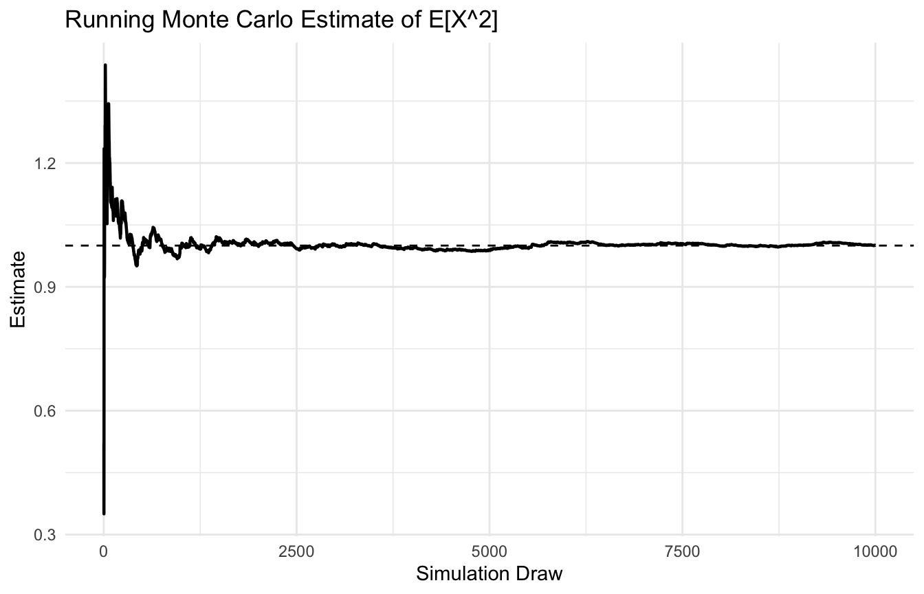
Since the true mean is 0, the estimate should be close to 0.

The key lesson is not the specific result. It is the idea that weighted simulation can approximate quantities under a target distribution without direct target sampling.


Importance Sampling Can Work Very Well or Very Badly

Importance sampling is elegant, but it can become unstable when the proposal distribution is poorly chosen.

Problems arise when:

  • the proposal puts too little mass where the target is large
  • the weights become highly variable
  • a few samples dominate the estimate

This is one reason importance sampling can struggle in high dimensions.

A good proposal distribution should resemble the target reasonably well.

That is one of the main practical lessons: importance sampling is powerful, but sensitive to proposal design.


MCMC Solves a Different Sampling Problem

When direct sampling is hard and importance sampling becomes unstable, another strategy is to construct a Markov chain whose long-run distribution is the target distribution.

This is the idea of Markov chain Monte Carlo, or MCMC.

Instead of drawing independent samples directly from the target, MCMC builds a dependent sequence of samples that eventually behaves like draws from the target.

This is extremely useful in Bayesian inference, where posterior distributions are often known only up to a proportionality constant.

MCMC lets us sample from such distributions without needing full analytic normalization.


Markov Chains Introduce Dependence Across Draws

A Markov chain is a stochastic process where the next state depends only on the current state, not the full past history.

That means MCMC samples are usually not independent.

This is a major difference from ordinary Monte Carlo or importance sampling.

The dependence does not make MCMC invalid. But it does mean we have to think about:

  • convergence,
  • mixing,
  • autocorrelation,
  • and effective sample size.

These are central practical concerns in MCMC-based inference.


Metropolis-Hastings Is One of the Classic MCMC Algorithms

One of the foundational MCMC algorithms is Metropolis-Hastings.

Its logic is:

  1. start at a current parameter value
  2. propose a new value from a proposal distribution
  3. compare how plausible the proposed value is relative to the current value
  4. accept or reject the proposal based on an acceptance probability

Over time, the chain explores the target distribution.

The beauty of Metropolis-Hastings is that it only needs the target distribution up to proportionality.

That makes it ideal for posterior distributions that are analytically awkward but easy to evaluate pointwise.


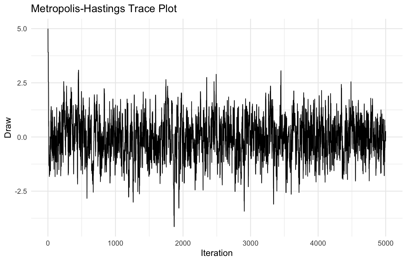
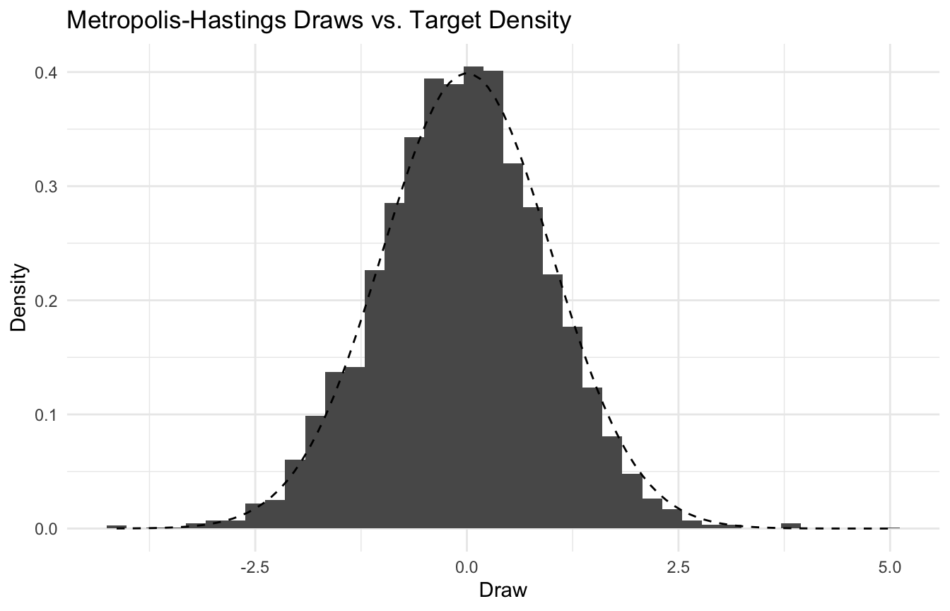
A Simple Metropolis-Hastings Example Makes MCMC Concrete

Suppose our target distribution is a standard normal density.

We will sample from it using a random-walk Metropolis-Hastings algorithm.

target_log_density <- function(x) {
  dnorm(x, mean = 0, sd = 1, log = TRUE)
}

n_iter <- 5000
chain <- numeric(n_iter)
chain[1] <- 5
proposal_sd <- 1

for (i in 2:n_iter) {
  current <- chain[i - 1]
  proposal <- rnorm(1, mean = current, sd = proposal_sd)
  
  log_alpha <- target_log_density(proposal) - target_log_density(current)
  
  if (log(runif(1)) < log_alpha) {
    chain[i] <- proposal
  } else {
    chain[i] <- current
  }
}

mh_df <- tibble::tibble(
  iter = 1:n_iter,
  draw = chain
)

mh_df |>
  dplyr::summarise(
    mean_draw = mean(draw),
    sd_draw = sd(draw)
  )
# A tibble: 1 × 2
  mean_draw sd_draw
      <dbl>   <dbl>
1   -0.0553   0.993

The empirical mean and standard deviation should be close to 0 and 1, respectively.


Trace Plots Help Diagnose Whether the Chain Is Exploring Well

One of the first things analysts inspect in MCMC is the trace plot (Gelman et al. 2013; Vehtari et al. 2021).

ggplot2::ggplot(mh_df, ggplot2::aes(x = iter, y = draw)) +
  ggplot2::geom_line(linewidth = 0.4) +
  ggplot2::labs(
    title = "Metropolis-Hastings Trace Plot",
    x = "Iteration",
    y = "Draw"
  ) +
  ggplot2::theme_minimal()

A trace plot helps assess whether the chain appears to be:

  • moving around the target region,
  • getting stuck,
  • drifting,
  • or mixing poorly.

It is not a perfect diagnostic, but it is one of the most useful first checks.


Histograms of the Chain Help Compare to the Target Distribution

A second useful check is to compare the empirical distribution of the chain to the known target shape.

ggplot2::ggplot(mh_df, ggplot2::aes(x = draw)) +
  ggplot2::geom_histogram(aes(y = after_stat(density)), bins = 40) +
  ggplot2::stat_function(fun = dnorm, args = list(mean = 0, sd = 1), linetype = 2) +
  ggplot2::labs(
    title = "Metropolis-Hastings Draws vs. Target Density",
    x = "Draw",
    y = "Density"
  ) +
  ggplot2::theme_minimal()

This gives a visual sense of whether the chain is reproducing the target distribution.


Acceptance Rate Matters in Metropolis-Hastings

One practical issue in Metropolis-Hastings is the acceptance rate.

If proposals are too small:

  • the chain accepts too often,
  • but explores slowly

If proposals are too large:

  • the chain rejects too often,
  • and can get stuck

The proposal scale therefore matters.

We can compute the acceptance rate.

accepted <- sum(diff(chain) != 0)
accept_rate <- accepted / (n_iter - 1)

tibble::tibble(
  acceptance_rate = accept_rate
)
# A tibble: 1 × 1
  acceptance_rate
            <dbl>
1           0.698

This is one of the most important tuning diagnostics in basic Metropolis-Hastings.


MCMC Is Especially Valuable in Bayesian Inference

One of the most important applications of MCMC is Bayesian inference.

In Bayesian workflows, the posterior often has the form:

\[ p(\theta \mid y) \propto p(y \mid \theta)p(\theta) \]

This posterior may be easy to evaluate up to proportionality, but hard to integrate or normalize exactly.

MCMC solves this by sampling from the posterior directly.

That allows analysts to approximate:

  • posterior means,
  • credible intervals,
  • posterior predictive distributions,
  • and tail probabilities

without needing closed-form formulas.

This is one reason MCMC became central to Bayesian statistics and Bayesian ML.


Monte Carlo Methods Matter for Risk Assessment Too

Monte Carlo methods are also extremely useful in risk modeling.

For example, in a biostatistical or health-systems setting, we may want to estimate:

  • the probability that demand exceeds capacity
  • the range of likely adverse event counts
  • the uncertainty in projected outcomes
  • or the tail risk of rare but consequential events

These are often best addressed through simulation.

A simple example is simulating patient demand under uncertain rates.

risk_df <- tibble::tibble(
  sim = 1:10000,
  daily_cases = rpois(10000, lambda = 18),
  severe_fraction = rbeta(10000, shape1 = 8, shape2 = 32)
) |>
  dplyr::mutate(
    severe_cases = daily_cases * severe_fraction
  )

risk_df |>
  dplyr::summarise(
    mean_severe_cases = mean(severe_cases),
    p95_severe_cases = quantile(severe_cases, 0.95),
    prob_over_6 = mean(severe_cases > 6)
  )
# A tibble: 1 × 3
  mean_severe_cases p95_severe_cases prob_over_6
              <dbl>            <dbl>       <dbl>
1              3.57             6.26      0.0635

This is a simple risk-assessment style Monte Carlo workflow. The same logic scales to much more complex models.


High Dimensions Make Everything Harder

A recurring theme in Monte Carlo methods is that high-dimensional problems are harder.

Why?

Because in high dimensions:

  • direct integration becomes difficult
  • importance weights can become unstable
  • chains can mix slowly
  • target geometry becomes more complex

This is one reason advanced MCMC methods and variational approximations became so important.

The basic ideas still matter, but the computational challenge grows quickly with dimension.

Understanding that difficulty helps explain why simulation-based inference remains an active research area.


Monte Carlo Methods Connect Statistics and AI Very Directly

Monte Carlo methods are one of the clearest bridges between classical statistics and modern AI.

They appear in:

  • Bayesian posterior inference
  • approximate integration
  • generative modeling
  • uncertainty estimation
  • simulation-based decision support
  • and reinforcement learning style sampling ideas

That is why they remain so important conceptually.

They show that randomness is not only noise. It can also be a computational tool for answering otherwise intractable questions.


A Practical Checklist for Applied Work

Before using Monte Carlo methods, ask:

  • What quantity am I trying to approximate?
  • Can I sample directly from the target, or do I need indirect methods?
  • Is importance sampling likely to be stable here?
  • Does MCMC mix well enough for the problem?
  • Have I checked trace plots and empirical summaries?
  • Is the dimensionality likely to create computational problems?
  • Am I using enough draws for the desired level of precision?

These questions often matter more than simply running the algorithm.


NoteWhere This Shows Up in AI/ML

Monte Carlo dropout — running inference through a neural network multiple times with different dropout masks active, then averaging the predictions — is one of the few practical uncertainty quantification methods deployed in production clinical AI systems, including deterioration prediction models in ICU settings where the width of the uncertainty interval determines whether an alert is escalated or suppressed. MCMC sampling underlies Bayesian trauma outcome models used to estimate 30-day mortality in DoDTR analysis, where the posterior over model coefficients quantifies how much the injury severity estimates depend on the prior when data from rare injury patterns are sparse. When dropout-based uncertainty is disabled at inference time — the standard PyTorch behavior unless explicitly overridden — the model produces single point estimates with no signal about when it is operating outside its training distribution.

Closing: Monte Carlo Methods Make Hard Inference Feasible

Monte Carlo methods remain essential because many important statistical and ML quantities are analytically difficult but simulation-friendly.

Basic Monte Carlo turns sampling into approximation. Importance sampling reweights simulation from a convenient proposal. MCMC builds dependent draws from otherwise intractable target distributions. Together, these methods make uncertainty quantification possible in problems that would otherwise be out of reach.

Monte Carlo methods matter because when exact inference is too hard, simulation lets us trade algebra for computation and still learn something useful.


Tip📚 Go Deeper: Bayesian Workflow Toolkit

This post is part of the Bayesian Workflow Toolkit — a companion reference with Monte Carlo integration templates, importance sampling code, Metropolis-Hastings scaffolds, and MCMC diagnostic tools.

→ Open the Bayesian Workflow Toolkit


Series Callout

Note

This post is part of a broader Applied Statistics for AI and Clinical Decision-Making Series:

  • Probability fundamentals for machine learning
  • Random variables and expectation
  • Common probability distributions
  • Central Limit Theorem
  • Law of Large Numbers
  • Sampling methods for Biostats and ML
  • Hypothesis testing in the age of AI
  • Confidence intervals
  • Maximum likelihood estimation
  • Bayesian inference
  • Linear regression
  • Logistic regression
  • Generalized linear models
  • Analysis of variance
  • Principal component analysis
  • Cluster analysis
  • Time series analysis
  • Survival analysis
  • Non-parametric methods
  • Bias-variance tradeoff
  • Regularization
  • Cross-validation
  • Information theory
  • Optimization techniques
  • Linear algebra basics
  • Calculus for ML
  • Monte Carlo methods
  • Dimensionality curse and reduction techniques
  • Model evaluation metrics
  • Ensemble methods

References

Gelman, Andrew, John B. Carlin, Hal S. Stern, David B. Dunson, Aki Vehtari, and Donald B. Rubin. 2013. Bayesian Data Analysis. 3rd ed. Chapman; Hall/CRC.
Hastings, W. K. 1970. “Monte Carlo Sampling Methods Using Markov Chains and Their Applications.” Biometrika 57 (1): 97–109. https://doi.org/10.1093/biomet/57.1.97.
Metropolis, Nicholas, Arianna W. Rosenbluth, Marshall N. Rosenbluth, Augusta H. Teller, and Edward Teller. 1953. “Equation of State Calculations by Fast Computing Machines.” The Journal of Chemical Physics 21 (6): 1087–92. https://doi.org/10.1063/1.1699114.
Owen, Art B. 2013. Monte Carlo Theory, Methods and Examples. Self-published. https://artowen.su.domains/mc/.
Robert, Christian P., and George Casella. 2004. Monte Carlo Statistical Methods. 2nd ed. Springer.
Vehtari, Aki, Andrew Gelman, Daniel Simpson, Bob Carpenter, and Paul-Christian Bürkner. 2021. “Rank-Normalization, Folding, and Localization: An Improved \(\widehat{R}\) for Assessing Convergence of MCMC.” Bayesian Analysis 16 (2): 667–718. https://doi.org/10.1214/20-BA1221.