Missing Data: From Diagnosis to Imputation to Sensitivity

Advanced Statistics for AI & Clinical Decision-Making — Lecture 1 of 4

Jonathan D. Stallings, PhD, MS

Data InDeed | dataindeed.org

2026-01-01

Missing data is not a cleaning problem. It is a modeling problem — and the model begins with why the data are missing.

What You’ll Learn Today

Post 01 Missing Data Mechanisms

• MCAR, MAR, MNAR
• Bias consequences
• Diagnostics

Post 02 Imputation Strategies

• Mean / median / KNN
• Multiple imputation (MICE)
• Pipeline integration

Post 03 Sensitivity Analysis

• Delta adjustment
• Pattern-mixture thinking
• Tipping-point analysis

This lecture is the gateway to advanced causal and observational methods. Every method in the next three lectures assumes you’ve dealt with missingness correctly — or at least honestly. Before we can talk about propensity scores or target trial emulation, we need to understand what our data is actually telling us when values are absent.

Part 1

Missing Data Mechanisms

MCAR, MAR, MNAR — the taxonomy that changes everything

The Same Missingness Rate, Three Different Problems

n <- 400
df_full <- tibble(
  severity = rnorm(n, 30, 12),   # ISS proxy
  outcome  = 5 + 0.4 * severity + rnorm(n, 0, 5)
)

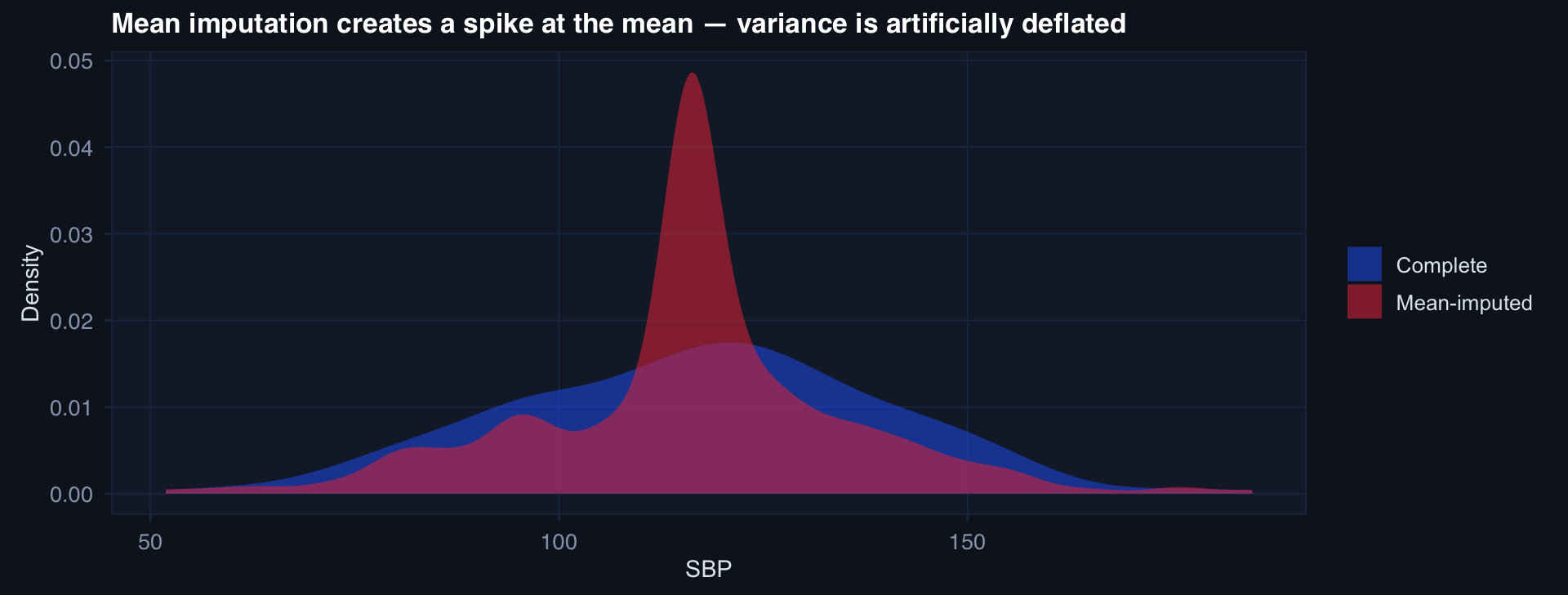
df_mcar <- df_full |> mutate(obs = ifelse(runif(n) > 0.3, outcome, NA))
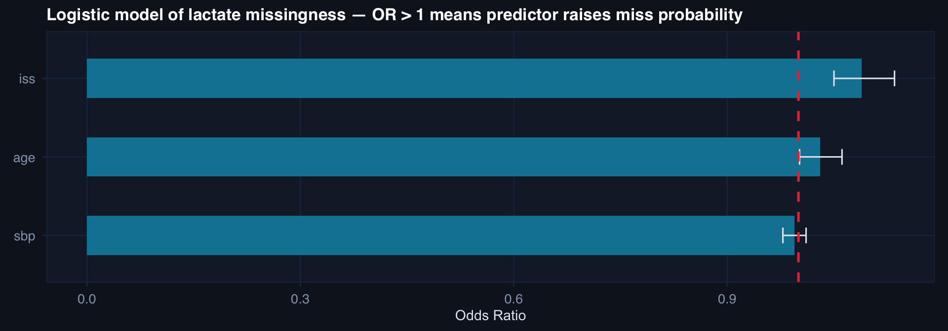
df_mar  <- df_full |> mutate(obs = ifelse(severity < 35 | runif(n) > 0.5, outcome, NA))
df_mnar <- df_full |> mutate(obs = ifelse(outcome < 20 | runif(n) > 0.4, outcome, NA))

# True mean
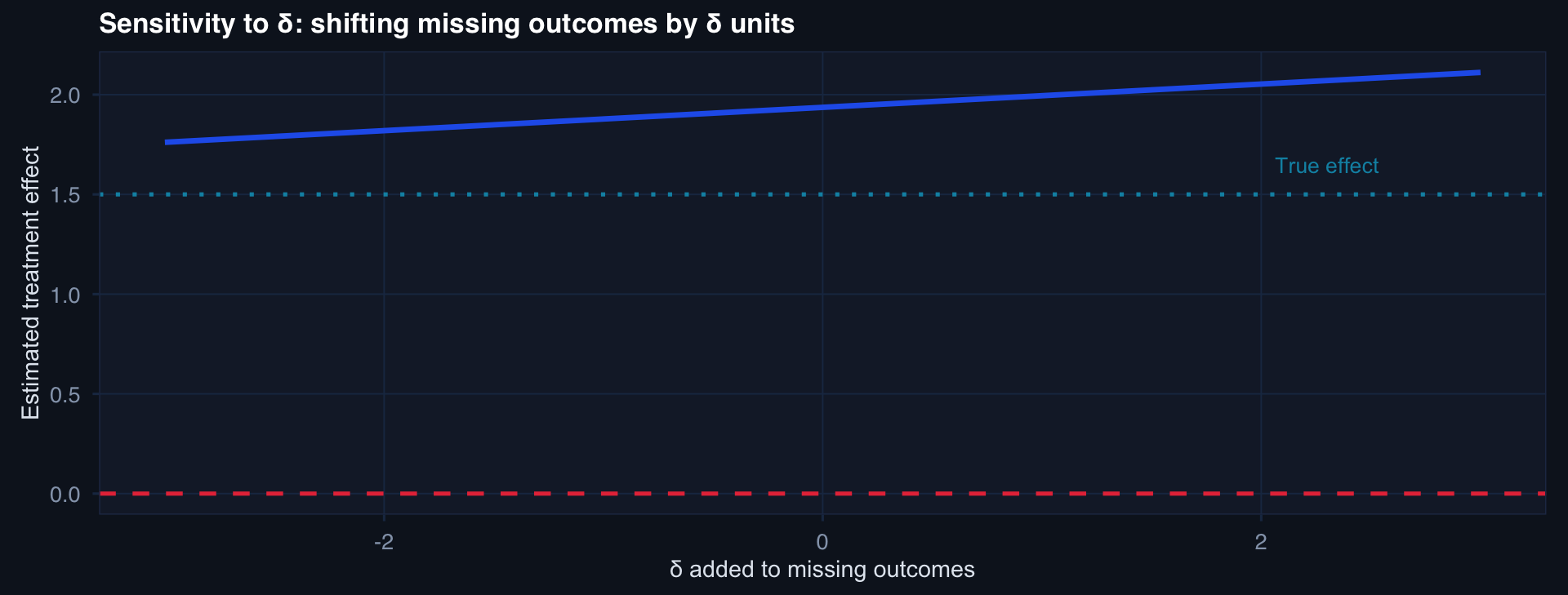
true_mean <- mean(df_full$outcome)

tibble(
  Mechanism = c("MCAR", "MAR", "MNAR"),
  `Observed mean` = c(mean(df_mcar$obs, na.rm=TRUE),
                      mean(df_mar$obs,  na.rm=TRUE),
                      mean(df_mnar$obs, na.rm=TRUE)),
  `True mean`     = true_mean,
  `% missing`     = c(mean(is.na(df_mcar$obs)),
                      mean(is.na(df_mar$obs)),
                      mean(is.na(df_mnar$obs))) * 100
) |>
  mutate(Bias = round(`Observed mean` - `True mean`, 2),
         across(where(is.numeric), round, 2))

# A tibble: 3 × 5
  Mechanism `Observed mean` `True mean` `% missing`  Bias
  <chr>               <dbl>       <dbl>       <dbl> <dbl>
1 MCAR                 17.7        17.6        28.2  0.15
2 MAR                  16.6        17.6        19.5 -1.01
3 MNAR                 16.4        17.6        13.8 -1.18

All three scenarios have ~30% missing. MCAR produces no bias. MAR produces recoverable bias (with the right model). MNAR produces bias that cannot be corrected without external assumptions.

The Three Mechanisms — Defined

MCAR Missing Completely At Random

Missingness is unrelated to any data — observed or unobserved.

Complete-case analysis is unbiased (just inefficient).

Example: Lab tube dropped randomly.

MAR Missing At Random

Missingness depends on observed variables, not the missing value itself.

Ignorable under likelihood-based methods. MICE works.

Example: GCS missing more often for high-ISS patients — but ISS is observed.

MNAR Missing Not At Random

Missingness depends on the unobserved value itself.

Not ignorable. Sensitivity analysis required.

Example: Lactate missing because it was never drawn — in the worst patients.

The clinical intuition here is crucial: MNAR is common in trauma registries precisely because sicker patients are less likely to have complete workups. A lab value that wasn’t drawn is not missing randomly — it’s missing because the patient was too unstable, or because the clinician already knew the answer. That’s MNAR.

Diagnosing Missingness: Is It MCAR?

# Missingness indicator regressed against observed predictors
df_diag <- tibble(
  iss      = rnorm(300, 28, 12),
  sbp      = rnorm(300, 110, 25),
  age      = rnorm(300, 35, 15)
) |> mutate(
  lactate_miss = rbinom(300, 1, plogis(-2 + 0.05*iss - 0.02*sbp))
)

fit_miss <- glm(lactate_miss ~ iss + sbp + age, data=df_diag, family=binomial)
broom::tidy(fit_miss, exponentiate=TRUE, conf.int=TRUE) |>
  filter(term != "(Intercept)") |>
  ggplot(aes(x=reorder(term, estimate), y=estimate)) +
  geom_col(fill="#0891b2", alpha=0.85, width=0.5) +
  geom_errorbar(aes(ymin=conf.low, ymax=conf.high), width=0.2, color="#e2e8f0") +
  geom_hline(yintercept=1, linetype=2, color="#e63946") +
  coord_flip() +
  labs(title="Logistic model of lactate missingness — OR > 1 means predictor raises miss probability",
       x=NULL, y="Odds Ratio") + theme_di()

ISS predicts missingness → not MCAR. If observed predictors explain missingness, you have MAR (or possibly MNAR). If nothing predicts missingness, you have evidence (not proof) of MCAR.

Part 2

Imputation Strategies

Filling gaps — the right way depends on the mechanism

The Imputation Hierarchy

Method	Mechanism assumption	Uncertainty captured	Use case
Complete-case	MCAR	No	Quick baseline
Mean/median	MCAR	No	Exploratory only
KNN	MAR	No	Prediction pipelines
MICE	MAR	Yes	Inference & modeling
Selection models	MNAR	Partial	Sensitivity analysis

The registry mistake: Most trauma analysts do complete-case analysis or mean imputation — fast, but silently biased. For any inference task (CPG compliance rates, mortality modeling), MICE is the minimum standard when data are MAR.

Why Mean Imputation Destroys Variance

n <- 300
sbp_true <- rnorm(n, 115, 22)
miss_idx  <- sample(n, 90)

sbp_obs   <- sbp_true; sbp_obs[miss_idx] <- NA
sbp_mean  <- sbp_obs;  sbp_mean[miss_idx] <- mean(sbp_obs, na.rm=TRUE)

tibble(
  Complete = sbp_true,
  `Mean-imputed` = sbp_mean
) |>
  pivot_longer(everything()) |>
  ggplot(aes(value, fill=name)) +
  geom_density(alpha=0.55, color=NA) +
  scale_fill_manual(values=c("#2563eb","#e63946")) +
  labs(title="Mean imputation creates a spike at the mean — variance is artificially deflated",
       x="SBP", y="Density", fill=NULL) + theme_di()

Mean imputation produces the right center but wrong spread. Confidence intervals built on mean-imputed data are too narrow — you’re seeing false precision.

MICE: Multiple Imputation by Chained Equations

The MICE algorithm (simplified):

1. Initialize missing values with mean imputation
2. For each variable with missingness, regress it on all others
3. Sample from the posterior predictive — don’t just take the point estimate
4. Repeat across m datasets → pool results with Rubin’s Rules

# Simulate MAR missing data and show distribution of imputed values
n <- 500
df_mice <- tibble(
  iss = rnorm(n, 28, 12),
  sbp = rnorm(n, 110, 22),
  gcs = rnorm(n, 13, 3)
) |> mutate(
  sbp_obs = ifelse(iss > 35 & runif(n) > 0.5, NA, sbp)
)

cat("Missing SBP:", sum(is.na(df_mice$sbp_obs)), "of", n, "(",
    round(100*mean(is.na(df_mice$sbp_obs)),1), "%)\n")

Missing SBP: 66 of 500 ( 13.2 %)

cat("Missingness model: high ISS raises miss probability (MAR)\n")

Missingness model: high ISS raises miss probability (MAR)

cat("True SBP mean:", round(mean(df_mice$sbp), 2),
    "\nObserved mean:", round(mean(df_mice$sbp_obs, na.rm=TRUE), 2))

True SBP mean: 109.16 
Observed mean: 108.75

Rubin’s Rules: Pool m imputed estimates as \(\bar{Q} = \frac{1}{m}\sum_{i=1}^m \hat{Q}_i\) with variance combining within- and between-imputation variance. m = 20–50 imputations is standard for 20–50% missing.

Part 3

Sensitivity Analysis for Missing Data

How fragile is your conclusion?

The Core Question: What Would Change Your Answer?

Sensitivity analysis doesn’t find the truth. It maps how far your conclusion can bend before it breaks.

Three tools:

• Delta adjustment — shift the missing values by δ and refit
• Pattern-mixture models — model separately by missingness group
• Tipping-point analysis — how extreme must the MNAR assumption be to reverse your result?

When it matters most:

Registry-based CPG compliance rates where non-documentation ≠ non-compliance.

Mortality models where the sickest patients have the most missing labs.

Any MNAR scenario where the missing value is related to the outcome.

Delta Adjustment: Shifting the Missing Values

# Simulate: true effect exists, but outcome is MNAR (high-outcome patients missing)
n <- 400
df_sa <- tibble(
  treatment = rbinom(n, 1, 0.5),
  outcome   = 2 + 1.5*treatment + rnorm(n, 0, 3),
  observed  = outcome < 6 | runif(n) > 0.35   # MNAR: high outcomes missing
)

# Delta grid: add delta to missing outcomes
delta_grid <- seq(-3, 3, by=0.5)
results <- sapply(delta_grid, function(d) {
  outcome_shifted <- df_sa$outcome
  outcome_shifted[!df_sa$observed] <- outcome_shifted[!df_sa$observed] + d
  coef(lm(outcome_shifted ~ treatment, data=df_sa))["treatment"]
})

tibble(delta=delta_grid, estimate=results) |>
  ggplot(aes(delta, estimate)) +
  geom_line(linewidth=1.2, color="#2563eb") +
  geom_hline(yintercept=0, linetype=2, color="#e63946") +
  geom_hline(yintercept=1.5, linetype=3, color="#0891b2") +
  annotate("text", x=2.3, y=1.65, label="True effect", color="#0891b2", size=3.5) +
  labs(title="Sensitivity to δ: shifting missing outcomes by δ units",
       x="δ added to missing outcomes", y="Estimated treatment effect") + theme_di()

The result stays positive across a wide δ range → relatively robust. If the null (0) is crossed at a small δ, the finding is fragile.

Tipping-Point Analysis

Tipping point: the minimum MNAR shift δ* that would change your conclusion (e.g., push the estimate past zero or past clinical significance).

Report: “Our finding would reverse only if missing outcomes were systematically X units higher than observed — an implausible shift given [clinical reasoning].”

Why this matters for communication:

Reviewers and commanders understand: > “The effect disappears only if we assume every missing lactate was 4 mmol/L above the patient’s true value.”

They don’t understand: > “We conducted a sensitivity analysis under MNAR.”

Practical table:

δ	Estimate	p-value	Conclusion
−2	0.8	0.09	Null
0	1.4	0.02	Positive
+2	2.1	0.001	Positive

δ=−2 is the tipping point → requires strong MNAR

Lecture 1 — Key Takeaways

Missing Data Mechanisms

• Mechanism determines bias, not missingness rate
• MCAR: unbiased complete-case analysis
• MAR: bias correctable with good imputation
• MNAR: requires sensitivity analysis — always
• Logistic missingness models outperform single tests

Imputation

• Mean imputation deflates variance → false precision
• KNN: good for prediction, no uncertainty
• MICE: gold standard for inference
• Always embed imputation in the CV pipeline

Sensitivity Analysis

• “Robust to sensitivity analysis” is a result, not an afterthought
• Delta adjustment is the simplest and most communicable
• Report the tipping point, not just the range tested
• Clinical judgment should bound the plausible δ

The meta-lesson: Before every model you build on registry data, ask: Why is this value missing? The answer determines whether your inference is valid — not the imputation method you chose.

Coming Up: Lecture 2

Causal Inference — From Correlation to Causation

Posts 04 & 05:

• Potential outcomes — Rubin’s causal model, ATE, ATT
• Randomization vs. observational data — why assignment mechanism matters
• Propensity scores — estimation, matching, weighting, balance diagnostics

Once the data are clean and missingness is handled, the next question is whether your estimates mean anything causally.

Read Before Lecture 2

• From Correlation to Causation
• Propensity Scores: Balancing the Scales