Trial Integrity: Blinding, Adaptive Designs & Pragmatic Trials

Design of Experiments — Lecture 3 of 4

Jonathan D. Stallings, PhD, MS

Data InDeed | dataindeed.org

2026-01-01

A trial that can’t adapt wastes information. A trial that isn’t blind contaminates it. A trial that ignores real-world care answers the wrong question.

What You’ll Learn Today

Post 07 Blinding & Expectation Bias

  • Single, double, triple blind
  • Placebo and sham controls
  • The placebo effect as outcome
  • When blinding fails

Post 08 Adaptive Trial Design

  • Interim analyses
  • Group-sequential stopping rules
  • Futility stopping
  • Adaptive randomization

Post 09 Pragmatic Trials

  • Efficacy vs. effectiveness
  • Cluster randomization
  • ICC and design effect
  • Intention-to-treat in practice

Part 1

Blinding & Expectation Bias

Protecting the comparison after randomization

What Randomization Does Not Fix

Randomization eliminates selection bias at baseline.

It does not prevent bias introduced after randomization:

Expectation bias sources:

  • Patients who know their assignment may report outcomes differently
  • Clinicians who know assignment may manage co-interventions differently
  • Outcome assessors who know assignment may grade outcomes differently
  • Data analysts unblinded to assignment may make different modeling choices

Each represents a distinct bias pathway — each requires a distinct blinding strategy.

Single blind: patient unaware

Double blind: patient + clinician unaware

Triple blind: + outcome assessor unaware

Quadruple blind: + analyst unaware (rare, but ideal for subjective endpoints)

Simulating Expectation Bias

n <- 300
df_blind <- tibble(
  trt  = rbinom(n, 1, 0.5),
  # True physiologic effect = 1.5 units
  phys = 1.5 * trt + rnorm(n, 0, 3),
  # Expectation bias: treated patients report 1.0 additional units if unblinded
  bias = ifelse(trt==1, rnorm(n, 1.0, 0.5), 0),
  # Observed outcomes
  y_blinded   = phys,
  y_unblinded = phys + bias
)

bind_rows(
  broom::tidy(lm(y_blinded   ~ trt, df_blind), conf.int=TRUE) |> mutate(Design="Blinded"),
  broom::tidy(lm(y_unblinded ~ trt, df_blind), conf.int=TRUE) |> mutate(Design="Unblinded")
) |> filter(term=="trt") |>
  ggplot(aes(estimate, Design, color=Design)) +
  geom_point(size=5) +
  geom_errorbarh(aes(xmin=conf.low, xmax=conf.high), height=0.2, linewidth=1) +
  geom_vline(xintercept=1.5, linetype=2, color="#94a3b8") +
  scale_color_manual(values=c("#e63946","#0891b2")) +
  annotate("text", x=1.65, y=2.4, label="True effect", color="#94a3b8", size=3.5) +
  labs(title="Expectation bias inflates the observed effect in unblinded trials",
       x="Estimated treatment effect (95% CI)", y=NULL) +
  theme_di() + theme(legend.position="none")

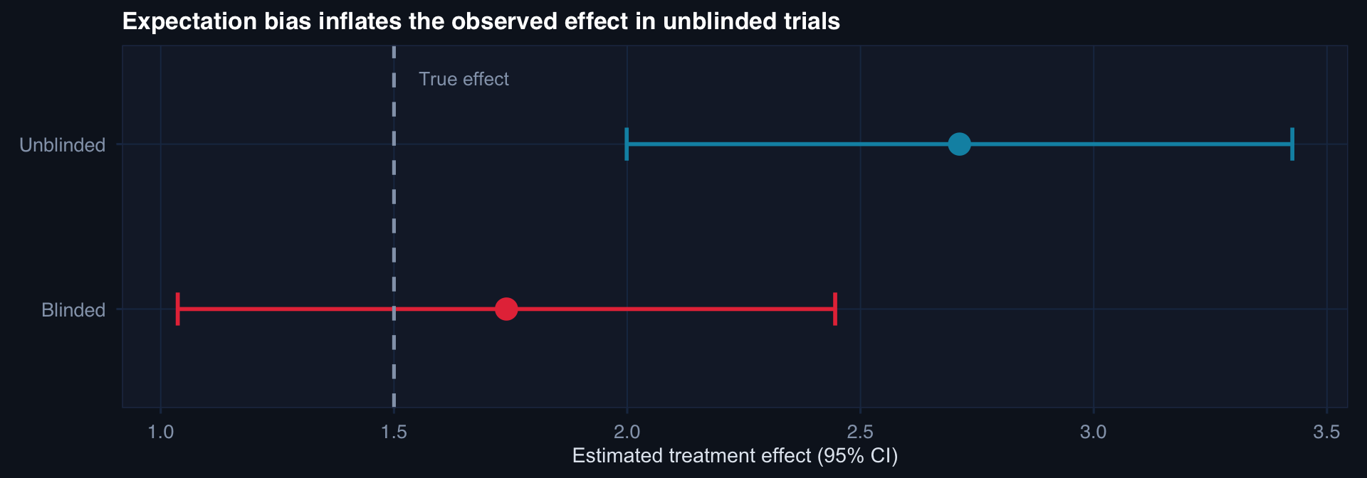
The unblinded estimate overstates the true effect by ~65%. In subjective outcomes (pain, function, quality of life), expectation bias can account for the majority of the observed effect.

When Blinding Is Difficult or Impossible

Hard to blind:

  • Surgical vs. medical interventions
  • Behavioral interventions
  • Dosing regimens with obvious side effects
  • Any intervention with observable characteristics

Strategies when full blinding fails:

  • Sham procedures (identical-appearing inactive intervention)
  • Centralized, blinded outcome adjudication
  • Objective endpoints (mortality, biomarkers, imaging)
  • Blinded statistical analysis plan pre-specified and locked

Trauma trial reality:

Tourniquet vs. no tourniquet cannot be blinded. DCS vs. definitive surgery cannot be blinded.

Design response: use hard objective outcomes (mortality, amputation, blood units transfused) that are less susceptible to expectation bias. Pre-register and lock the primary endpoint before unblinding.

Part 2

Adaptive Trial Design

Learning from data without compromising validity

The Fixed-Design Problem

A standard trial collects all n observations, then analyzes once.

Two failure modes:

Early success ignored: The treatment clearly works after 40% enrollment. The trial continues for 18 more months, exposing 60% of patients to inferior care (or to a less effective treatment).

Futility ignored: After 60% enrollment, the effect is clearly near zero. The trial continues, burning resources, patient time, and clinician goodwill.

Adaptive designs pre-specify decision rules for:

  • Early stopping for efficacy — evidence already strong
  • Early stopping for futility — effect clearly negligible
  • Sample size re-estimation — adjust n based on interim variance
  • Adaptive randomization — shift allocation toward better arm

Group-Sequential Stopping Rules

# Simulate a group sequential trial: 4 interim + 1 final look
# O'Brien-Fleming boundaries (conservative early, lenient late)
n_looks <- 5
info_fractions <- seq(0.2, 1.0, by=0.2)
# O'Brien-Fleming critical values (approximate)
obf_alpha <- c(4.56, 3.23, 2.63, 2.28, 2.04) / sqrt(n_looks)

# Simulate trial data with true treatment effect
n_total <- 200
trt  <- rep(0:1, each=n_total/2)
y    <- 10 - 1.8*trt + rnorm(n_total, 0, 4)

# Compute running z-statistic at each look
look_n <- floor(n_total * info_fractions)
z_stats <- sapply(look_n, function(k) {
  idx <- 1:k
  m1 <- mean(y[trt==1 & seq_along(trt) %in% idx])
  m0 <- mean(y[trt==0 & seq_along(trt) %in% idx])
  s  <- sd(y[seq_along(y) %in% idx])
  (m1 - m0) / (s * sqrt(2/k))
})

tibble(fraction=info_fractions, z=abs(z_stats), boundary=obf_alpha) |>
  ggplot(aes(fraction)) +
  geom_ribbon(aes(ymin=0, ymax=boundary), fill="#253554", alpha=0.6) +
  geom_line(aes(y=boundary), color="#e63946", linewidth=1.2, linetype=2) +
  geom_line(aes(y=z), color="#0891b2", linewidth=1.3) +
  geom_point(aes(y=z), color="#22d3ee", size=4) +
  annotate("text", x=0.85, y=3.0, label="O'Brien-Fleming\nboundary", color="#e63946", size=3.2) +
  annotate("text", x=0.55, y=1.2, label="Observed |Z|", color="#0891b2", size=3.2) +
  labs(title="Group-sequential trial: |Z| crosses boundary at final look → stop for efficacy",
       x="Information fraction (proportion of data observed)", y="|Z statistic|") +
  theme_di()

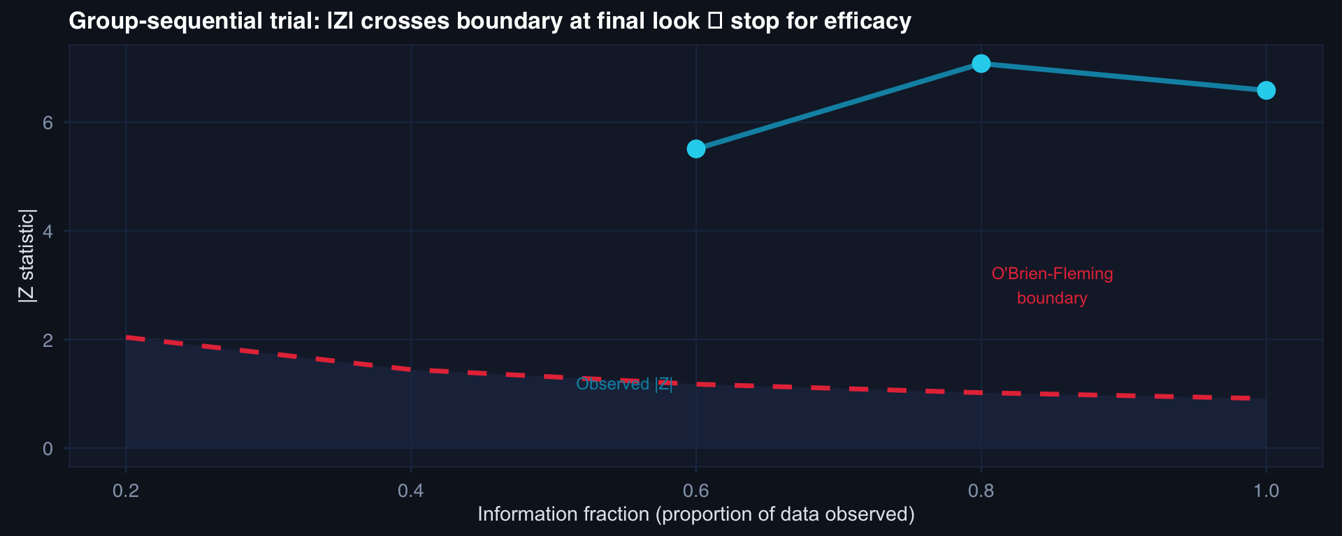
O’Brien-Fleming: boundary is high early (conservative) and converges to ~1.96 at the final look. Preserves type I error at α = 0.05 across all looks.

Adaptive Randomization: Shifting Toward the Better Arm

Response-adaptive randomization (RAR):

As interim data accumulates, allocation probability shifts toward the arm showing better outcomes.

Benefit: Fewer patients assigned to the inferior treatment.

Cost: Groups become unequal in size → reduced power. Temporal confounding if patient characteristics drift. Operational complexity.

Appropriate when:

  • Outcomes observable quickly (not 6-month endpoints)
  • Strong ethical imperative to minimize inferior-arm exposure
  • Feasibility for complex adaptive logistics exists

Trauma application:

RAR most appropriate for:

  • Fluid resuscitation dosing
  • Analgesic protocol comparison
  • Where immediate outcomes (hemodynamic stabilization) guide allocation

Least appropriate for:

  • 90-day mortality endpoints (slow feedback)
  • Small n where adaptation adds more noise than signal

Part 3

Pragmatic Trial Design

Answering questions about real-world effectiveness

Efficacy vs. Effectiveness: Two Different Questions

Dimension Explanatory (Efficacy) Pragmatic (Effectiveness)
Question Can this work? Does this work in practice?
Setting Controlled, specialized centers Routine care settings
Participants Narrow eligibility, homogeneous Broad eligibility, diverse
Adherence Enforced, monitored closely As-delivered, real-world
Outcome Mechanistic or surrogate Patient-centered, operational
Analysis Per-protocol Intention-to-treat
Generalizability Lower Higher

Military example: An efficacy trial of TXA in controlled hemorrhagic shock model → can it reduce mortality under ideal conditions? A pragmatic trial across DoDTR-enrolled facilities → does TXA delivered under real prehospital conditions improve outcomes at the system level?

Cluster Randomization: When Individual Randomization Is Impossible

# Demonstrate ICC and design effect in cluster-randomized data
n_clusters <- 20; n_per <- 25
ICC <- 0.12  # within-facility correlation

# Simulate clustered binary outcomes
cluster_effects <- rnorm(n_clusters, 0, sqrt(ICC))
df_cluster <- expand_grid(cluster=1:n_clusters, patient=1:n_per) |>
  mutate(
    trt   = ifelse(cluster <= n_clusters/2, 1, 0),
    u_clust = cluster_effects[cluster],
    y     = rbinom(n(), 1, plogis(-1.5 + 0.6*trt + u_clust))
  )

# Show within-cluster similarity
df_cluster |>
  group_by(cluster, trt) |>
  summarise(rate=mean(y), .groups="drop") |>
  ggplot(aes(factor(cluster), rate, fill=factor(trt))) +
  geom_col(alpha=0.85) +
  scale_fill_manual(values=c("#2563eb","#e63946"),
                    labels=c("Control facility","Treatment facility")) +
  labs(title=paste0("Cluster-randomized trial: ICC = ", ICC,
                    " → design effect ≈ ", round(1 + (n_per-1)*ICC, 2),
                    "× larger required n"),
       x="Facility (cluster)", y="Outcome rate", fill=NULL) +
  theme_di() + theme(axis.text.x=element_blank())

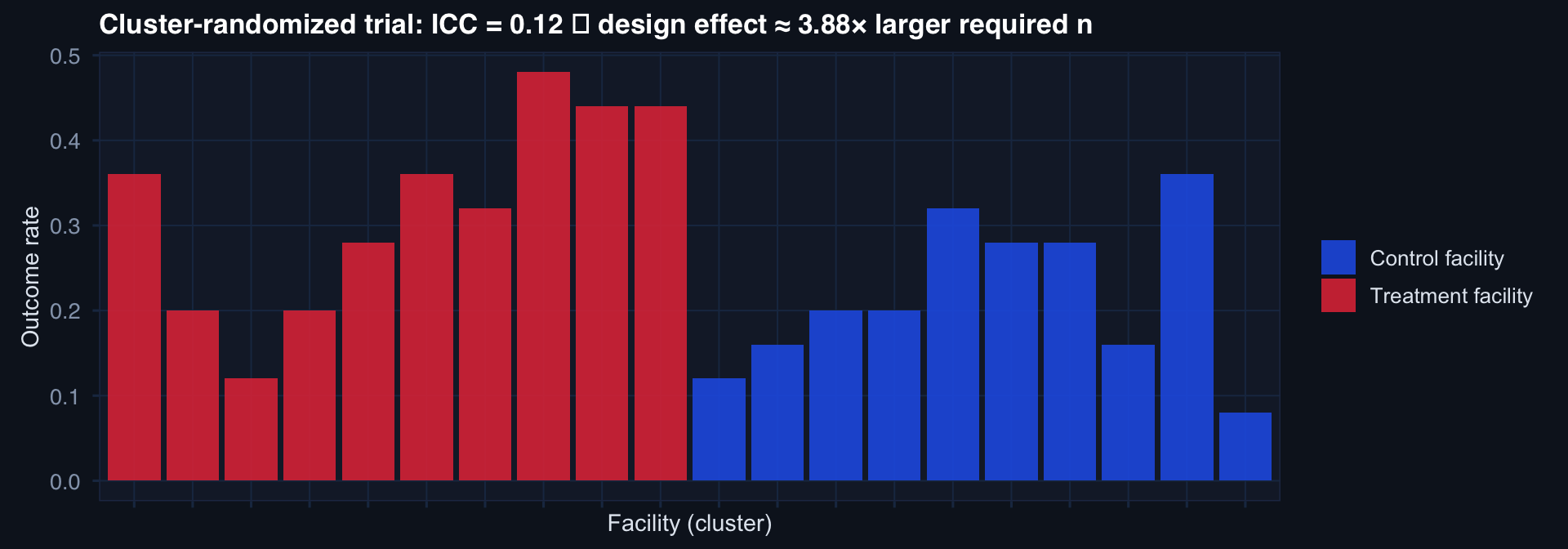
Design effect (DEFF) = \(1 + (m-1) \cdot \text{ICC}\) where \(m\) = cluster size.

ICC = 0.12, m = 25 → DEFF ≈ 4.0 → need 4× as many patients as individual randomization would require. Underestimating ICC is the most common power error in cluster trials.

Intention-to-Treat: The Pragmatic Analysis Standard

ITT principle: Analyze patients in the group they were assigned to, regardless of what they actually received.

Why: Departures from assigned treatment are part of real-world effectiveness. ITT answers: “What happens if we implement this policy?” — not “What happens if everyone follows it perfectly?”

Modified ITT (mITT): Excludes patients who never received any treatment — a common and acceptable restriction, but must be pre-specified.

Per-protocol analysis: Analyzes only adherent patients. Complementary — not a replacement for ITT.

When per-protocol diverges from ITT:

If PP shows a larger effect than ITT, the treatment works — but implementation/adherence is a barrier.

If ITT shows no effect but PP does, the system failed to deliver the intervention, not the intervention itself.

Report both. Explain the divergence. It’s often the most interesting finding.

Lecture 3 — Key Takeaways

Blinding

  • Randomization ≠ blinding — they address different bias sources
  • Single/double/triple: patient, clinician, assessor
  • Unblindable trials → objective endpoints + locked analysis plan
  • Report blinding method and integrity checks (CONSORT)

Adaptive Designs

  • Pre-specify all interim analysis rules in the protocol
  • O’Brien-Fleming: conservative early, standard threshold late
  • Futility stopping is as important as efficacy stopping
  • RAR: ethical gain at cost of power and complexity

Pragmatic Trials

  • Effectiveness ≠ efficacy — different question, different design
  • Cluster randomization for system-level interventions
  • ICC drives sample size: underestimating it is the #1 error
  • ITT is the primary analysis; PP is supplementary

The meta-lesson: Blinding, adaptation, and pragmatic framing are not add-ons — they are design decisions that determine whether the trial answers its stated question in a defensible way.

Coming Up: Lecture 4

Quasi-Experimental Designs & Design Strategy

Post 10 + synthesis:

  • Interrupted time series — using time as the comparison
  • Difference-in-differences — adding a control group to ITS
  • Regression discontinuity — exploiting threshold-based assignment
  • Choosing the right design — a decision framework across all 10 posts