Building Better Models: Bias, Variance & Validation

Applied Statistics for AI & Clinical Decision-Making — Lecture 8 of 10

Jonathan D. Stallings, PhD, MS

Data InDeed | dataindeed.org

2026-01-01

A model that memorizes training data has learned nothing.

What You’ll Learn Today

Post 20 Bias-Variance

• The fundamental tradeoff
• Underfitting vs. overfitting
• Decomposing MSE

Post 21 Regularization

• Ridge (L2)
• Lasso (L1)
• Elastic net

Post 22 Cross-Validation

• k-fold CV
• Leave-one-out
• Selecting hyperparameters

Part 1

The Bias-Variance Tradeoff

The fundamental tension in model complexity

Decomposing Prediction Error

\[E[\text{MSE}] = \text{Bias}^2 + \text{Variance} + \text{Irreducible noise}\]

Bias — error from wrong assumptions (underfitting)

• Model is too simple
• Misses real patterns
• High training error AND test error

Variance — error from sensitivity to training data (overfitting)

• Model is too complex
• Memorizes noise
• Low training error, HIGH test error

Irreducible noise — cannot be reduced by any model

Registry analogy:

A linear model for ISS → mortality may be biased (relationship is not linear at extremes).

A 500-node neural network on 200 patients is high variance — it memorizes those 200 patients but won’t generalize.

The Bias-Variance Curve

tibble(
  complexity = 1:10,
  bias_sq = (5 / (1:10))^2,
  variance = (0.3 * (1:10))^2,
) |>
  dplyr::mutate(total = bias_sq + variance + 4) |>
  tidyr::pivot_longer(-complexity) |>
  ggplot(aes(complexity, value, color=name, linewidth=name)) +
  geom_line() +
  scale_color_manual(values=c("bias_sq"="#e63946","variance"="#2563eb",
                              "total"="#1b2e4b")) +
  scale_linewidth_manual(values=c("bias_sq"=0.9,"variance"=0.9,"total"=1.4)) +
  labs(title="Bias² + Variance + noise = total expected error",
       x="Model complexity", y="Error", color=NULL, linewidth=NULL) + theme_di()

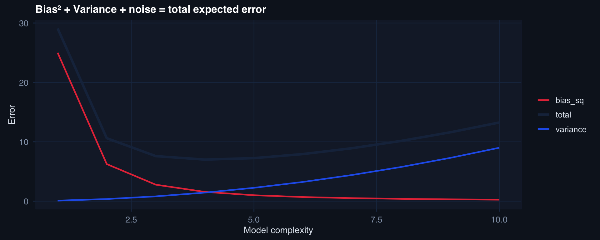
The sweet spot: find the complexity that minimizes total error — not bias alone or variance alone.

Part 2

Regularization

Penalizing complexity to prevent overfitting

Ridge (L2) and Lasso (L1)

Ridge: minimize \(\text{RSS} + \lambda \sum_j \beta_j^2\)

Lasso: minimize \(\text{RSS} + \lambda \sum_j |\beta_j|\)

Property	Ridge	Lasso
Shrinks coefficients	Yes	Yes
Sets coefficients to zero	No	Yes
Variable selection	No	Yes
Best when	All features matter	Many irrelevant features
Solution	Closed form	Coordinate descent

Elastic Net = combination of both: \(\alpha \cdot \text{Lasso} + (1-\alpha) \cdot \text{Ridge}\)

Lasso Path: Automatic Feature Selection

n <- 200; p <- 20
X <- matrix(rnorm(n*p), n, p)
# Only first 4 features truly predict outcome
beta_true <- c(2,-1.5,1,-0.8, rep(0,16))
y <- X %*% beta_true + rnorm(n)

fit_lasso <- glmnet(X, y, alpha=1)
plot(fit_lasso, xvar="lambda", label=TRUE,
     main="Lasso coefficient paths — features shrink to zero")

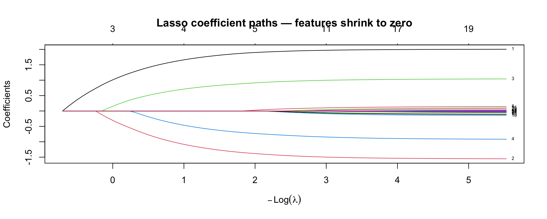
As λ increases (more regularization), coefficients are forced to zero. The 4 true predictors (1–4) survive longest.

The lasso path plot is one of the most instructive plots in modern statistical learning. You can see which features the model considers important (survive at high λ) vs. noise (zeroed out early). In a trauma registry with 200 variables, lasso might zero out 180 of them, leaving the 20 that actually matter.

Choosing λ with Cross-Validation

cv_lasso <- cv.glmnet(X, y, alpha=1, nfolds=10)
plot(cv_lasso)

cat("Optimal λ:", round(cv_lasso$lambda.min, 4),
    "\nλ 1-SE rule:", round(cv_lasso$lambda.1se, 4))

Optimal λ: 0.0489 
λ 1-SE rule: 0.1495

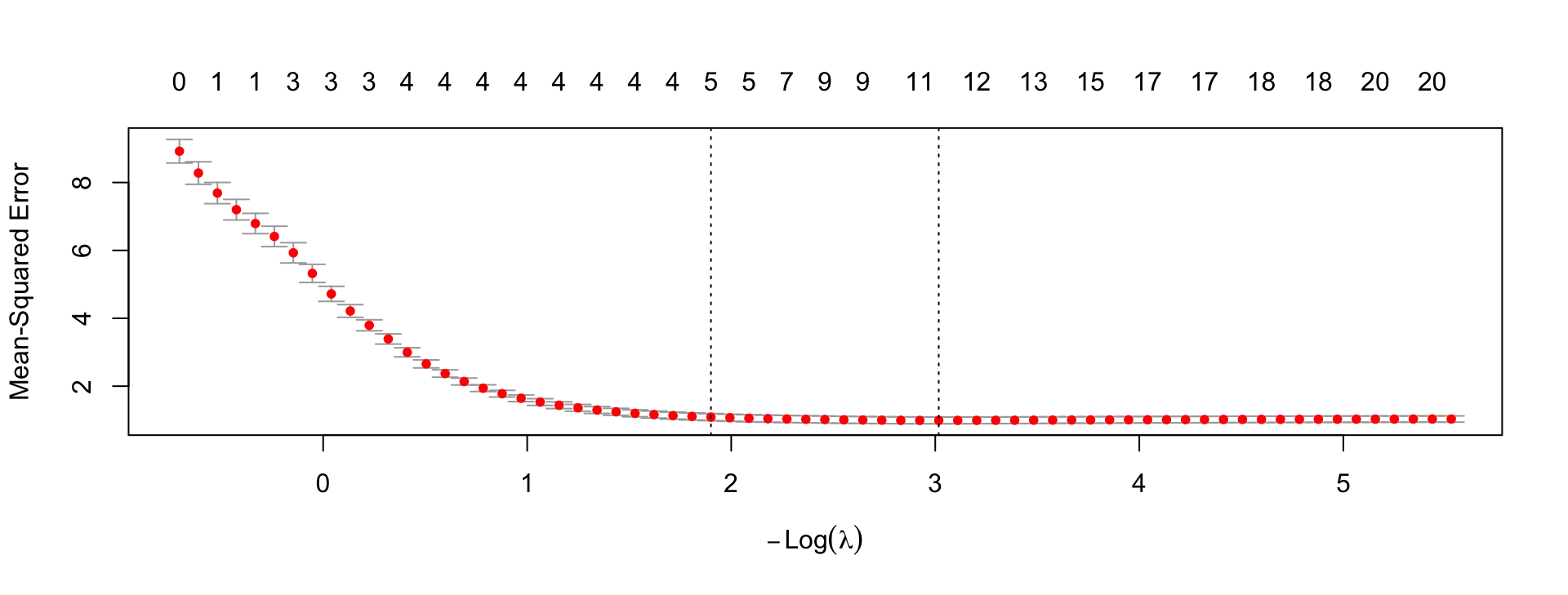
1-SE rule: prefer the simplest model within 1 standard error of the minimum CV error — favors parsimony.

Part 3

Cross-Validation

The honest way to estimate generalization error

k-Fold Cross-Validation

1. Divide data into k roughly equal folds
2. For each fold i = 1...k:

   - Train on all folds except i
   - Evaluate on fold i
3. Average performance across all k test folds

manual_kfold <- function(df, k=5) {
  folds <- sample(rep(1:k, length.out=nrow(df)))
  sapply(1:k, function(i) {
    train <- df[folds != i, ]; test <- df[folds == i, ]
    fit <- lm(los ~ iss + sbp, data=train)
    sqrt(mean((test$los - predict(fit, test))^2))
  })
}
df_cv <- tibble(iss=rnorm(200,28,12), sbp=rnorm(200,110,20),
                los=2+0.4*iss-0.02*sbp+rnorm(200,0,4))
rmse_folds <- manual_kfold(df_cv)
tibble(fold=1:5, RMSE=round(rmse_folds,2)) |> print()

# A tibble: 5 × 2
   fold  RMSE
  <int> <dbl>
1     1  4.34
2     2  4.8 
3     3  3.42
4     4  3.69
5     5  3.69

cat("CV RMSE:", round(mean(rmse_folds),3), "±", round(sd(rmse_folds),3))

CV RMSE: 3.99 ± 0.569

Leave-One-Out vs. k-Fold

	LOO-CV	k-Fold (k=5 or 10)
Bias	Very low	Low
Variance	High	Lower
Computation	Expensive (n fits)	Cheap (k fits)
Best for	Small datasets	Most situations

General recommendation: 5- or 10-fold CV is the standard. LOO when n < 50.

Temporal validation for registry models: In clinical practice, always validate forward in time. Split by enrollment date — train on 2019-2022, test on 2023-2024. This catches data drift that k-fold CV (which ignores time) cannot detect.

Lecture 8 — Key Takeaways

Bias-Variance

• MSE = Bias² + Variance + noise
• Underfitting (high bias) = model too simple
• Overfitting (high variance) = model too complex
• Goal: find complexity that minimizes total error

Regularization

• Ridge: shrinks all coefficients
• Lasso: zeroes out irrelevant features (selection)
• Elastic net: combines both
• λ chosen by cross-validation

Cross-Validation

• k-fold: standard approach (k=5 or 10)
• LOO: for very small n
• Temporal CV: required for longitudinal registry data
• CV error = honest estimate of generalization

The meta-lesson: A model evaluated only on training data tells you nothing about how it will perform on future patients.

Coming Up: Lecture 9

Model Evaluation & Ensembles

Posts 29, 30, 17:

• Metrics That Matter — AUC, F1, calibration, clinical utility
• Ensembles — bagging, boosting, random forests
• Time Series — autoregression, seasonality, forecasting

Read Before Lecture 9

• Metrics That Matter
• Ensembles: Supercharging Stats
• Time Series Stats