LLN in Action: Building Reliable ML Models from Noisy Data
Applied Statistics
Law of Large Numbers
An applied introduction to the Law of Large Numbers, convergence of sample means, and why larger samples stabilize estimates in statistics and machine learning.
It formalizes a principle that many analysts intuitively trust:
as we observe more data, averages become more stable.
That idea is foundational in statistics, clinical research, and machine learning.
If a process has a true average outcome, then repeated observations from that process should eventually produce a sample average that gets close to the truth.
This is why larger studies tend to produce more reliable estimates. It is why model performance estimated on small samples can be unstable. And it is why training on more data often improves the credibility of empirical summaries.
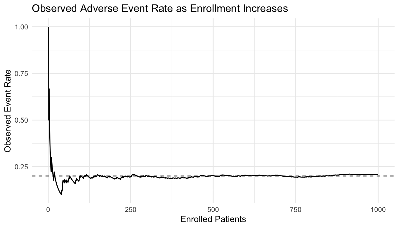
In machine learning, the Law of Large Numbers helps explain why empirical risk can approximate population risk. In biostatistics, it helps explain why trial estimates stabilize as enrollment grows.
This post introduces the Law of Large Numbers through intuition, simulation, and applied examples.
We will focus on:
what the Law of Large Numbers says,
the difference between weak and strong forms,
how convergence looks in code,
and why the idea matters for reliable ML and clinical inference.
The Law of Large Numbers does not eliminate randomness. It makes randomness average out in predictable ways.
The Law of Large Numbers Explains Why Averages Settle Down
Individual observations are noisy.
A single patient outcome may differ from expectation. A single model prediction may be wrong. A single device reading may be erratic. A single trial participant may not reflect the broader population.
But when we average across many observations, the noise begins to cancel.
That is the intuition behind the Law of Large Numbers.
If observations are generated from a stable process with a finite mean, then the sample average tends to approach the true population mean as the sample size increases (DeGroot and Schervish 2012; Casella and Berger 2002).
This is one of the central reasons statistics works at all.
Without some form of averaging stability, inference would be much harder.
What the Law of Large Numbers Actually Says
Let (X_1, X_2, , X_n) be random variables with common mean ().
Define the sample mean as:
\[
\bar{X}_n = \frac{1}{n}\sum_{i=1}^{n} X_i
\]
The Law of Large Numbers says that as \(n\) grows, the sample mean \(\bar{X}_n\) converges to the true mean \(\mu\).
In plain language:
small samples can fluctuate a lot,
but large samples tend to average out those fluctuations.
This does not mean every large sample is perfect. It means the average becomes increasingly reliable in a probabilistic sense.
Weak vs. Strong LLN: Same Destination, Different Kind of Guarantee
There are two commonly discussed forms of the Law of Large Numbers.
Weak Law of Large Numbers
The weak LLN says that the sample mean converges to the true mean in probability.
That means:
for any fixed tolerance, the probability that the sample mean differs substantially from the true mean goes to zero as (n) increases.
This is a probabilistic guarantee.
Strong Law of Large Numbers
The strong LLN says that the sample mean converges to the true mean almost surely.
That is a stronger statement.
It means that with probability 1, the sequence of sample means eventually settles toward the true mean.
In practice, both tell a similar story for applied work:
more data makes averages more trustworthy.
But mathematically, the strong law gives a stronger mode of convergence.
The LLN Is About Convergence of Averages, Not Elimination of Variability
A common misunderstanding is that the Law of Large Numbers says randomness disappears.
It does not.
Randomness remains in the raw observations.
What changes is that the average becomes more stable.
This distinction matters.
A dataset of individual patient outcomes may remain heterogeneous even in a very large sample. A model may still make variable predictions case-by-case.
What stabilizes is the summary quantity: the sample mean, empirical proportion, or average loss.
That is why the LLN is so relevant to estimation and machine learning objectives.
A Simple Simulation Makes the LLN Visible
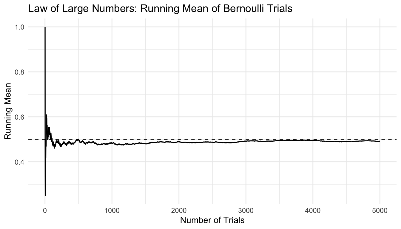
The easiest way to understand the LLN is to simulate repeated observations and track the running average.
We will begin with a simple example using coin flips coded as 1 for heads and 0 for tails.
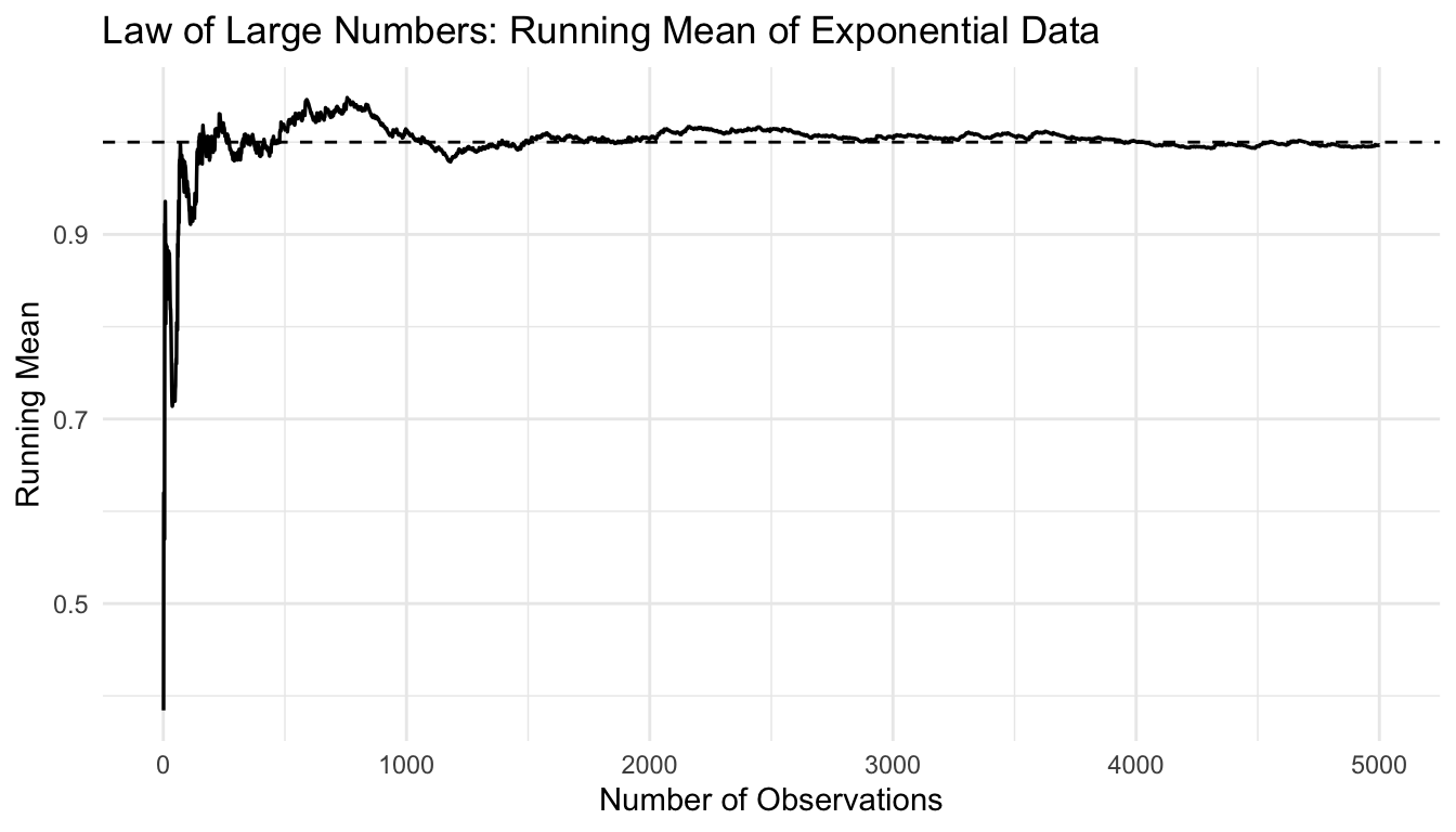
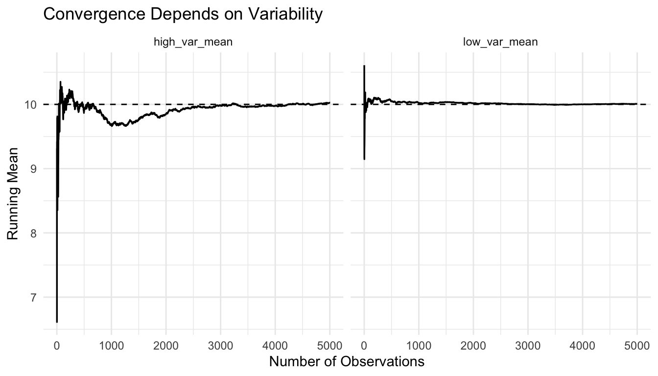
The target is the same in both cases, but the noisier process takes longer to settle.
LLN in Model Evaluation: Why Averaging Across Folds Helps
In applied ML, performance estimates based on a single split can be unstable.
That is one reason analysts use:
repeated train/test splits,
cross-validation,
repeated cross-validation,
bootstrap summaries.
Averaging across repeated evaluations does not remove all uncertainty, but it often improves stability.
That logic is closely aligned with the LLN.
As more evaluation replications are included, the average performance estimate becomes more dependable than any single split.
This is especially important when communicating model performance to decision-makers.
The LLN Is Also a Governance Idea
At a practical level, the Law of Large Numbers supports a governance principle:
do not overinterpret noisy early averages.
This matters in:
interim trial reviews,
early model validation,
pilot deployments,
monitoring dashboards,
and sequential reporting.
Small-sample summaries can appear dramatic. Some of that drama is just variance.
The LLN reminds us that reliability often comes from repeated accumulation, not from the first striking number.
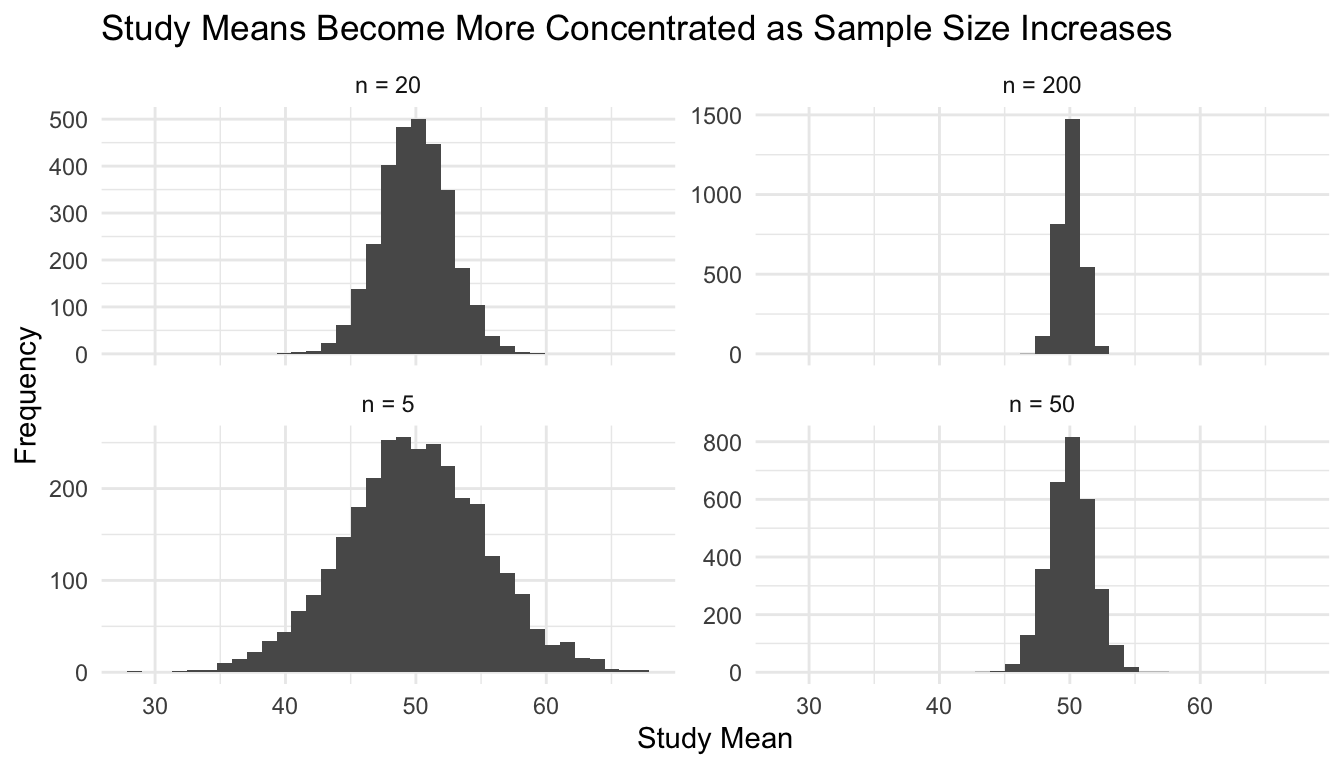
A Simulation of Repeated Study Means
Another useful way to understand the LLN is to compare study-level means across increasing sample sizes.
Below, we simulate many studies and examine how the study means become more concentrated as sample size grows.
simulate_study_means <-function(n, n_reps =3000) { tibble::tibble(rep =1:n_reps,study_mean =replicate(n_reps, mean(rnorm(n, mean =50, sd =12))),n =paste0("n = ", n) )}study_means_df <- dplyr::bind_rows(simulate_study_means(5),simulate_study_means(20),simulate_study_means(50),simulate_study_means(200))ggplot2::ggplot(study_means_df, ggplot2::aes(x = study_mean)) + ggplot2::geom_histogram(bins =35) + ggplot2::facet_wrap(~ n, scales ="free_y") + ggplot2::labs(title ="Study Means Become More Concentrated as Sample Size Increases",x ="Study Mean",y ="Frequency" ) + ggplot2::theme_minimal()
This reinforces the same lesson: larger samples produce more stable averages.
A Practical Checklist for Applied Work
Before trusting a sample average, ask:
Is the sample size large enough for the quantity to stabilize?
Is the data-generating process reasonably representative?
Are observations independent enough for the average to behave well?
Could high variance or heavy tails slow convergence?
Am I averaging a meaningful quantity, such as loss, rate, or response?
Have I confused stability of the average with correctness of the model?
These questions improve both modeling and interpretation.
NoteWhere This Shows Up in AI/ML
AUC estimates reported from validation sets of 200–300 patients — typical for many published military health AI studies — have confidence intervals wide enough to be clinically meaningless; the LLN guarantees that a sample AUC converges to the true AUC, but convergence is slow enough that a reported AUC of 0.81 on n=250 could easily reflect a true AUC anywhere from 0.72 to 0.88. Deployment decisions based on small-sample AUC estimates at military treatment facilities have led to adoption of models that degraded to near-chance performance in prospective use, a failure that the LLN directly predicts and that adequate sample size planning would prevent.
Closing: Reliability Comes from Repetition, Not Wishful Thinking
The Law of Large Numbers is one of the key reasons analysts can learn from data.
It tells us that repeated observations, under appropriate conditions, allow sample averages to approach true population quantities.
That idea supports:
clinical estimation,
trial monitoring,
model evaluation,
empirical risk minimization,
and the consistency of many familiar estimators.
It does not remove bias. It does not rescue poor data. And it does not guarantee that every large dataset is informative.
But it does explain why averaging across enough observations can transform noise into something interpretable.
The Law of Large Numbers is one of the quiet foundations of reliable science and machine learning: it explains why enough data can make averages worth trusting.
This post is part of the Prediction Modeling Toolkit — a companion reference with convergence diagnostics, empirical risk estimation templates, and sample-size sensitivity checks.
Casella, George, and Roger L. Berger. 2002. Statistical Inference. 2nd ed. Duxbury.
DeGroot, Morris H., and Mark J. Schervish. 2012. Probability and Statistics. 4th ed. Pearson.
Hastie, Trevor, Robert Tibshirani, and Jerome Friedman. 2009. The Elements of Statistical Learning: Data Mining, Inference, and Prediction. 2nd ed. Springer.
James, Gareth, Daniela Witten, Trevor Hastie, and Robert Tibshirani. 2021. An Introduction to Statistical Learning: With Applications in R. 2nd ed. Springer.
Wasserman, Larry. 2004. All of Statistics: A Concise Course in Statistical Inference. Springer.