Mastering Sampling: From Biostats Surveys to ML Data Prep

Applied Statistics
Sampling
A practical introduction to simple random sampling, stratified sampling, and bootstrap resampling for biostatistics and machine learning workflows.
Published

August 15, 2023

Modified

June 9, 2026

Executive Summary

Sampling is one of the most practical ideas in statistics (DeGroot and Schervish 2012; Lohr 2021).

In theory, we would like complete information about a population. In practice, we usually work with subsets:

  • a subset of patients,
  • a subset of sites,
  • a subset of records,
  • a subset of training examples,
  • or repeated resamples from the same observed dataset.

That makes sampling more than a data collection topic. It is a core design principle for both biostatistics and machine learning.

The way we sample data affects:

  • bias,
  • variance,
  • representativeness,
  • class balance,
  • uncertainty estimation,
  • and model evaluation.

This post introduces three important sampling approaches:

  • simple random sampling,
  • stratified sampling,
  • bootstrap resampling.

Along the way, we will connect them to:

  • survey logic,
  • clinical and biostatistical reasoning,
  • cross-validation and ML data preparation,
  • and bootstrap confidence intervals for regression.

Sampling is not just about choosing data. It is about shaping what conclusions your model is allowed to learn.


Sampling Sits Between the Population and the Model

A model never learns directly from the full abstract population.

It learns from data that were:

  • observed,
  • recorded,
  • selected,
  • filtered,
  • cleaned,
  • and often resampled.

That means sampling choices influence not only estimation, but also what patterns a model can even detect.

In biostatistics, this is obvious in surveys, trials, and registries.

In machine learning, it appears through:

  • train/test splits,
  • cross-validation folds,
  • class-balancing strategies,
  • bootstrap performance estimation,
  • bagging and ensemble workflows.

Sampling is therefore not a preliminary nuisance. It is part of the inferential engine.


Simple Random Sampling Is the Baseline Design

The most basic sampling scheme is simple random sampling.

Under simple random sampling, every unit in the population has an equal chance of being selected (Lohr 2021).

This design is attractive because it is conceptually clean and often analytically convenient.

To illustrate, we will create a synthetic “population” with a binary subgroup, a continuous predictor, and a continuous outcome.

library(dplyr)
library(tibble)
library(ggplot2)
library(tidyr)

n_pop <- 10000

population_df <- tibble::tibble(
  id = 1:n_pop,
  group = sample(c("Group A", "Group B"), size = n_pop, replace = TRUE, prob = c(0.75, 0.25)),
  x = rnorm(n_pop, mean = 50, sd = 10)
) |>
  dplyr::mutate(
    y = 10 + 0.8 * x + dplyr::if_else(group == "Group B", 6, 0) + rnorm(n_pop, 0, 8)
  )

population_df |>
  dplyr::summarise(
    pop_mean_x = mean(x),
    pop_mean_y = mean(y)
  )
# A tibble: 1 × 2
  pop_mean_x pop_mean_y
       <dbl>      <dbl>
1       50.1       51.5

Now take a simple random sample.

srs_df <- population_df |>
  dplyr::slice_sample(n = 400)

srs_df |>
  dplyr::summarise(
    sample_mean_x = mean(x),
    sample_mean_y = mean(y)
  )
# A tibble: 1 × 2
  sample_mean_x sample_mean_y
          <dbl>         <dbl>
1          50.6          51.8

Simple random sampling works well when the population is reasonably homogeneous or when subgroup representation is not a major concern.

But that is not always the case.


Stratified Sampling Helps Preserve Important Subgroups

Sometimes a simple random sample underrepresents smaller but important groups.

That is where stratified sampling becomes useful.

In stratified sampling, we divide the population into strata, then sample within each stratum (Lohr 2021).

This can improve representation and sometimes improve estimator precision.

Below, we take an equal-size stratified sample by group.

strat_df <- population_df |>
  dplyr::group_by(group) |>
  dplyr::slice_sample(n = 200) |>
  dplyr::ungroup()

strat_df |>
  dplyr::count(group)
# A tibble: 2 × 2
  group       n
  <chr>   <int>
1 Group A   200
2 Group B   200

Compare the group composition of the population, the simple random sample, and the stratified sample.

composition_df <- dplyr::bind_rows(
  population_df |>
    dplyr::count(group) |>
    dplyr::mutate(source = "Population"),
  srs_df |>
    dplyr::count(group) |>
    dplyr::mutate(source = "Simple Random Sample"),
  strat_df |>
    dplyr::count(group) |>
    dplyr::mutate(source = "Stratified Sample")
) |>
  dplyr::group_by(source) |>
  dplyr::mutate(pct = n / sum(n)) |>
  dplyr::ungroup()

composition_df
# A tibble: 6 × 4
  group       n source                 pct
  <chr>   <int> <chr>                <dbl>
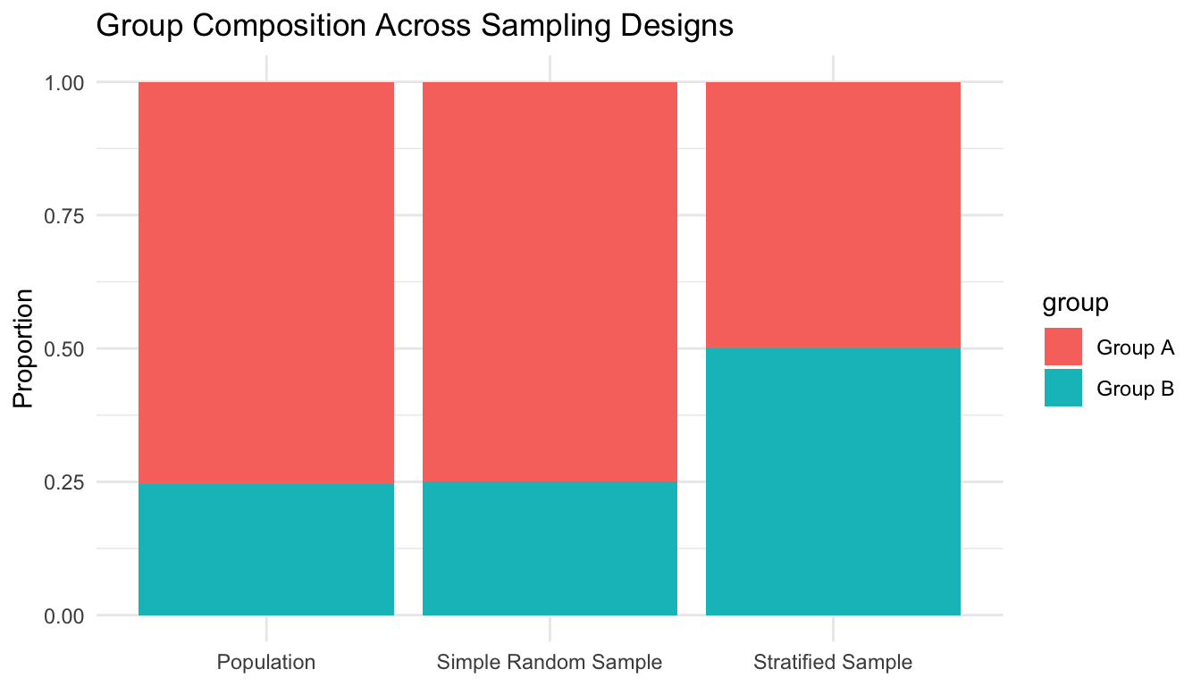
1 Group A  7538 Population           0.754
2 Group B  2462 Population           0.246
3 Group A   300 Simple Random Sample 0.75 
4 Group B   100 Simple Random Sample 0.25 
5 Group A   200 Stratified Sample    0.5  
6 Group B   200 Stratified Sample    0.5  
ggplot2::ggplot(composition_df, ggplot2::aes(x = source, y = pct, fill = group)) +
  ggplot2::geom_col(position = "stack") +
  ggplot2::labs(
    title = "Group Composition Across Sampling Designs",
    x = NULL,
    y = "Proportion"
  ) +
  ggplot2::theme_minimal()

This is especially relevant when rare subgroups matter scientifically or operationally.


Sampling Design Affects Bias and Variance

Sampling is not only about representation. It also influences bias and variance.

At a high level:

  • bias reflects systematic deviation from the truth,
  • variance reflects instability across repeated samples.

A poor sampling strategy can produce biased estimates. A small but unbiased sampling design may still have high variance.

We can compare repeated simple random samples and repeated stratified samples for estimating the population mean of y.

estimate_mean_srs <- function(pop_df, n = 400) {
  pop_df |>
    dplyr::slice_sample(n = n) |>
    dplyr::summarise(est = mean(y)) |>
    dplyr::pull(est)
}

estimate_mean_strat <- function(pop_df, n_per_group = 200) {
  pop_df |>
    dplyr::group_by(group) |>
    dplyr::slice_sample(n = n_per_group) |>
    dplyr::ungroup() |>
    dplyr::summarise(est = mean(y)) |>
    dplyr::pull(est)
}

true_mean_y <- mean(population_df$y)

sampling_compare_df <- tibble::tibble(
  rep = 1:1000,
  srs_est = replicate(1000, estimate_mean_srs(population_df, n = 400)),
  strat_est = replicate(1000, estimate_mean_strat(population_df, n_per_group = 200))
) |>
  tidyr::pivot_longer(
    cols = c(srs_est, strat_est),
    names_to = "method",
    values_to = "estimate"
  )

sampling_compare_df |>
  dplyr::group_by(method) |>
  dplyr::summarise(
    mean_estimate = mean(estimate),
    bias = mean(estimate) - true_mean_y,
    variance = var(estimate),
    .groups = "drop"
  )
# A tibble: 2 × 4
  method    mean_estimate    bias variance
  <chr>             <dbl>   <dbl>    <dbl>
1 srs_est            51.5 -0.0155    0.353
2 strat_est          53.1  1.60      0.330

This helps show that sampling strategy is connected to estimator behavior, not just bookkeeping.


Stratified Sampling Matters in Biostats and in ML

In biostatistics, stratification is familiar from:

  • age strata,
  • treatment arms,
  • site categories,
  • severity groups,
  • sex-based or risk-based subgroup reporting.

In ML, the same logic appears in:

  • stratified train/test splits,
  • stratified cross-validation,
  • balanced batch construction,
  • imbalanced outcome handling.

If the outcome class is rare, naive random splitting can create unstable evaluation sets.

Stratified resampling often improves comparability by preserving class proportions across folds.

That is not just convenient. It improves interpretability.


Bootstrap Resampling Treats the Observed Sample as a Population Proxy

The bootstrap is different from sampling from a known population (Efron and Tibshirani 1993).

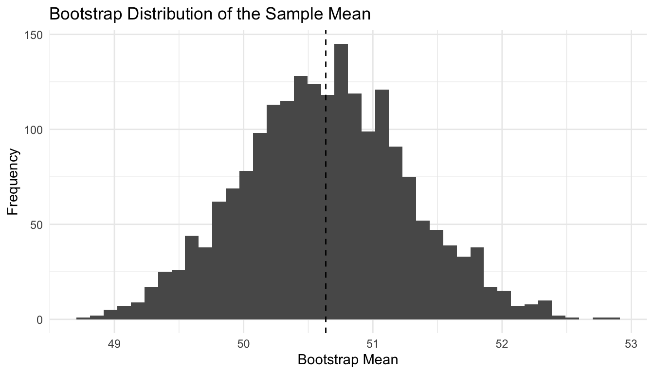
Instead, it repeatedly samples with replacement from the observed dataset (Efron and Tibshirani 1993).

The key idea is:

if the observed sample is a reasonable stand-in for the underlying population, then repeated resampling from it can approximate the sampling distribution of a statistic.

This is one of the most useful tools in modern applied statistics.

It helps estimate:

  • standard errors,
  • confidence intervals,
  • optimism in model performance,
  • uncertainty in regression coefficients,
  • and stability of predictive metrics.

We will start with a bootstrap estimate for the mean.

observed_df <- population_df |>
  dplyr::slice_sample(n = 300)

boot_means <- tibble::tibble(
  rep = 1:2000,
  boot_mean = replicate(
    2000,
    observed_df |>
      dplyr::slice_sample(n = nrow(observed_df), replace = TRUE) |>
      dplyr::summarise(est = mean(y)) |>
      dplyr::pull(est)
  )
)

boot_means |>
  dplyr::summarise(
    bootstrap_mean = mean(boot_mean),
    bootstrap_se = sd(boot_mean),
    ci_lower = quantile(boot_mean, 0.025),
    ci_upper = quantile(boot_mean, 0.975)
  )
# A tibble: 1 × 4
  bootstrap_mean bootstrap_se ci_lower ci_upper
           <dbl>        <dbl>    <dbl>    <dbl>
1           50.6        0.647     49.4     51.9

Bootstrapping Makes Uncertainty Visible

A major benefit of the bootstrap is that it gives a direct empirical approximation to the sampling distribution of a statistic.

ggplot2::ggplot(boot_means, ggplot2::aes(x = boot_mean)) +
  ggplot2::geom_histogram(bins = 40) +
  ggplot2::geom_vline(xintercept = mean(observed_df$y), linetype = 2) +
  ggplot2::labs(
    title = "Bootstrap Distribution of the Sample Mean",
    x = "Bootstrap Mean",
    y = "Frequency"
  ) +
  ggplot2::theme_minimal()

This is especially useful when analytic standard errors are inconvenient, unavailable, or less trustworthy under complex modeling settings.


A Bootstrap Confidence Interval for a Regression Coefficient

A practical way to connect this to ML and applied modeling is to bootstrap a regression coefficient.

We will fit a simple linear model:

\[ y = \beta_0 + \beta_1 x + \epsilon \]

and bootstrap the slope estimate.

reg_df <- population_df |>
  dplyr::slice_sample(n = 500)

fit_lm <- lm(y ~ x, data = reg_df)

summary(fit_lm)$coefficients
             Estimate Std. Error   t value     Pr(>|t|)
(Intercept) 14.369793 1.82171477  7.888059 1.959530e-14
x            0.751831 0.03546234 21.200833 1.441387e-71

Now bootstrap the slope.

boot_slopes <- tibble::tibble(
  rep = 1:2000,
  slope = replicate(
    2000,
    {
      boot_df <- reg_df |>
        dplyr::slice_sample(n = nrow(reg_df), replace = TRUE)
      coef(lm(y ~ x, data = boot_df))[["x"]]
    }
  )
)

boot_slopes |>
  dplyr::summarise(
    mean_slope = mean(slope),
    se_slope = sd(slope),
    ci_lower = quantile(slope, 0.025),
    ci_upper = quantile(slope, 0.975)
  )
# A tibble: 1 × 4
  mean_slope se_slope ci_lower ci_upper
       <dbl>    <dbl>    <dbl>    <dbl>
1      0.754   0.0361    0.684    0.825
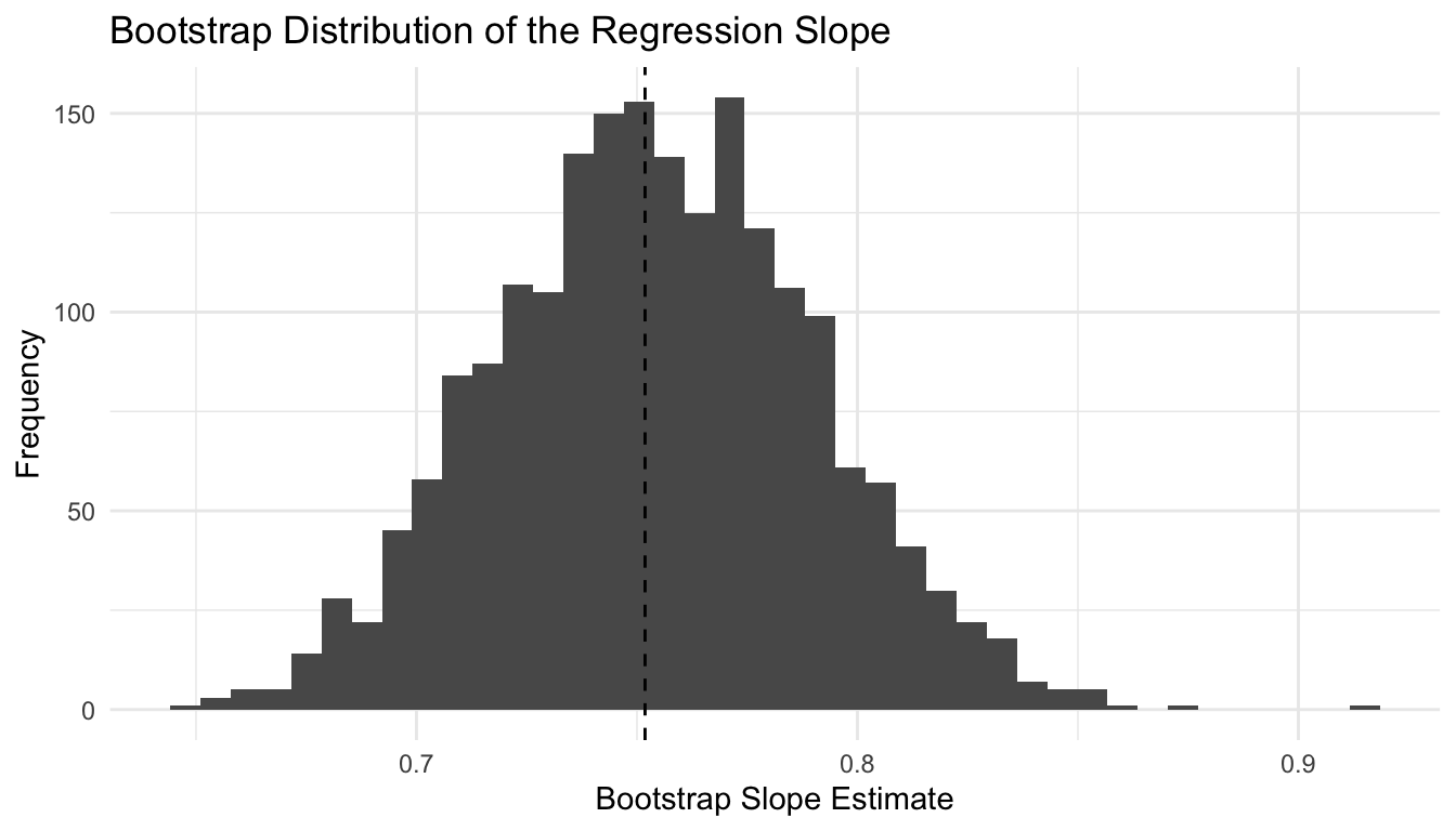
ggplot2::ggplot(boot_slopes, ggplot2::aes(x = slope)) +
  ggplot2::geom_histogram(bins = 40) +
  ggplot2::geom_vline(xintercept = coef(fit_lm)[["x"]], linetype = 2) +
  ggplot2::labs(
    title = "Bootstrap Distribution of the Regression Slope",
    x = "Bootstrap Slope Estimate",
    y = "Frequency"
  ) +
  ggplot2::theme_minimal()

This gives a bootstrap-based confidence interval for the slope without relying only on model-based normal theory.


Why Bootstrapping Matters for ML

Bootstrapping is deeply connected to machine learning practice.

It helps with:

  • uncertainty quantification,
  • model stability assessment,
  • optimism correction,
  • ensemble learning,
  • bagging,
  • and repeated performance estimation.

Random forests, for example, rely on bootstrap-like resampling of training data for tree construction.

More generally, resampling gives analysts a way to ask:

how much would this result change if the sample had been slightly different?

That is a powerful question in any predictive workflow.


Sampling Also Matters for Class Imbalance

Many ML problems involve rare outcomes.

Examples include:

  • fraud detection,
  • adverse event prediction,
  • rare disease classification,
  • mortality prediction,
  • equipment failure.

In those settings, naive random sampling can create distorted training sets or unstable validation results.

Common responses include:

  • stratified splitting,
  • oversampling minority classes,
  • undersampling majority classes,
  • weighted losses,
  • synthetic resampling approaches.

Not all of these are “sampling” in the classical survey sense, but they are all part of the broader problem of how data are selected, balanced, and presented to the model.


Cross-Validation Is Also a Sampling Workflow

Cross-validation is often described as a model evaluation strategy, but it is also a sampling design.

Each split selects:

  • a training subset,
  • a validation subset,
  • and a repeated structure for averaging performance.

That means cross-validation inherits many of the same concerns:

  • representativeness,
  • fold stability,
  • outcome balance,
  • dependence,
  • and estimator variability.

Seen this way, cross-validation is not separate from sampling theory. It is one of its modern applied extensions.


Bias-Variance Tradeoffs Often Show Up Through Resampling

Resampling methods also help analysts reason about bias and variance.

For example:

  • a small training sample may yield high-variance model estimates,
  • an imbalanced split may bias evaluation,
  • bootstrap distributions can reveal estimator instability,
  • repeated folds can expose sensitivity to data partitioning.

This is one reason resampling is so important in model governance.

It helps move beyond a single-number estimate toward a distributional understanding of performance.


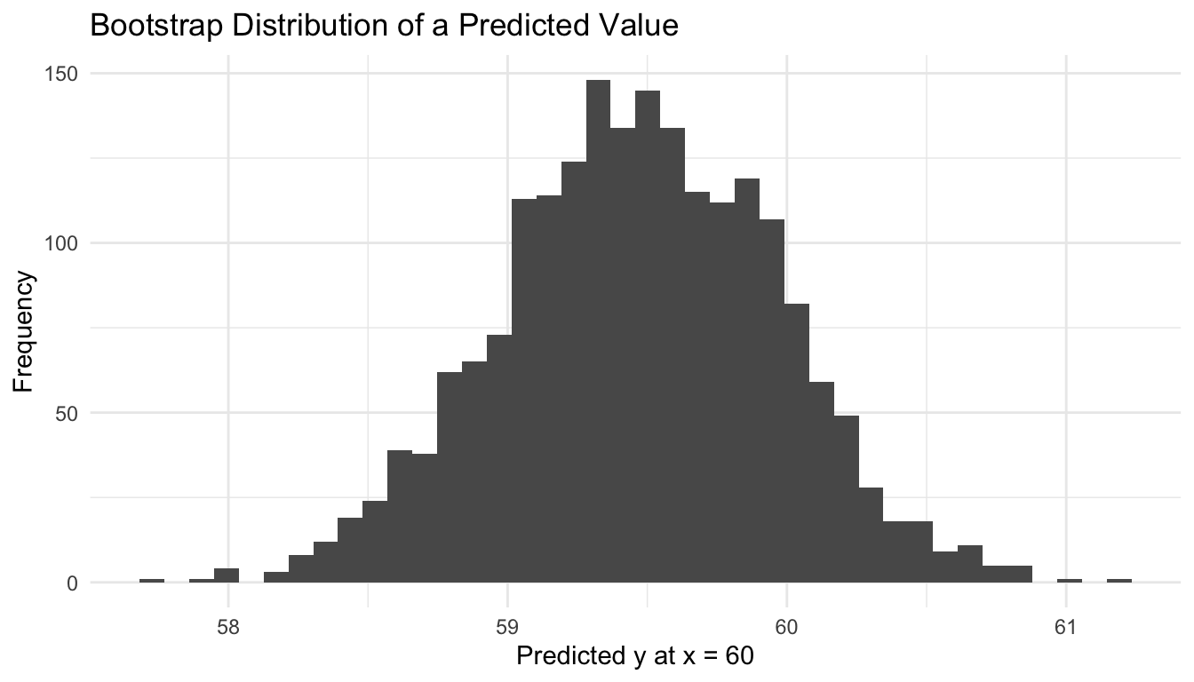
A Simple Bootstrap Prediction Example

We can push the regression example one step further by generating predicted values at a fixed x and bootstrapping that prediction.

x0 <- 60

boot_preds <- tibble::tibble(
  rep = 1:2000,
  pred = replicate(
    2000,
    {
      boot_df <- reg_df |>
        dplyr::slice_sample(n = nrow(reg_df), replace = TRUE)
      fit <- lm(y ~ x, data = boot_df)
      predict(fit, newdata = data.frame(x = x0))
    }
  )
)

boot_preds |>
  dplyr::summarise(
    mean_pred = mean(pred),
    ci_lower = quantile(pred, 0.025),
    ci_upper = quantile(pred, 0.975)
  )
# A tibble: 1 × 3
  mean_pred ci_lower ci_upper
      <dbl>    <dbl>    <dbl>
1      59.5     58.5     60.4
ggplot2::ggplot(boot_preds, ggplot2::aes(x = pred)) +
  ggplot2::geom_histogram(bins = 40) +
  ggplot2::labs(
    title = "Bootstrap Distribution of a Predicted Value",
    x = "Predicted y at x = 60",
    y = "Frequency"
  ) +
  ggplot2::theme_minimal()

This is often more tangible for readers because it connects uncertainty directly to an estimated model output.


Sampling Does Not Fix Bad Data

It is important not to romanticize resampling.

No sampling method can fully rescue:

  • systematic measurement error,
  • unmeasured confounding,
  • selection bias,
  • severe distribution shift,
  • or poor variable definitions.

Bootstrap intervals, for example, quantify uncertainty conditional on the observed sample. They do not automatically correct structural flaws in the data-generating process.

This is especially important in clinical and operational settings.

More resampling does not equal more truth if the source data are fundamentally biased.


A Practical Checklist for Applied Work

Before choosing a sampling strategy, ask:

  • Am I trying to estimate a population quantity, preserve subgroup structure, or quantify uncertainty?
  • Is subgroup representation important?
  • Is the outcome imbalanced?
  • Do I need analytic standard errors, or would bootstrap intervals be more useful?
  • Is my evaluation sensitive to how I split the data?
  • Am I using resampling to understand instability, or pretending it solves bias?

These questions usually matter as much as the model itself.

NoteWhere This Shows Up in AI/ML

Bootstrap resampling is the standard method for constructing confidence intervals around AUC, Brier score, and calibration slope for clinical prediction models — the FDA’s guidance on AI/ML-based software as a medical device explicitly recommends reporting these interval estimates rather than point metrics, because point AUC alone cannot support a deployment decision. The DoDTR suffers from systematic sampling bias toward patients who survived long enough to reach a trauma center with registry infrastructure, meaning any model trained on DoDTR without correcting for this survivorship bias will underestimate mortality risk for the most severely injured casualties — exactly the patients where decision support matters most.


Closing: Sampling Is Part of the Model, Not Just the Data Prep

Sampling methods shape what we learn from data.

Simple random sampling gives a clean baseline. Stratified sampling protects representation where subgroup structure matters. Bootstrap resampling helps quantify uncertainty when closed-form answers are difficult or unavailable.

In both biostatistics and machine learning, these are not side topics.

They affect:

  • estimation,
  • fairness,
  • model evaluation,
  • uncertainty quantification,
  • and how confidently we communicate results.

Reliable models do not come only from clever algorithms. They also come from thoughtful sampling, careful resampling, and honest uncertainty assessment.


Tip📚 Go Deeper: Real-World Evidence Toolkit

This post is part of the Real-World Evidence Toolkit — a companion reference with sampling scheme templates, bootstrap confidence interval code, and survey-weighted analysis scaffolds.

→ Open the Real-World Evidence Toolkit


Series Callout

Note

This post is part of a broader Applied Statistics for AI and Clinical Decision-Making Series:

  • Probability fundamentals for machine learning
  • Random variables and expectation
  • Common probability distributions
  • Central Limit Theorem
  • Law of Large Numbers
  • Sampling methods for Biostats and ML
  • Hypothesis testing in the age of AI
  • Confidence intervals
  • Maximum likelihood estimation
  • Bayesian inference
  • Linear regression
  • Logistic regression
  • Generalized linear models
  • Analysis of variance
  • Principal component analysis
  • Cluster analysis
  • Time series analysis
  • Survival analysis
  • Non-parametric methods
  • Bias-variance tradeoff
  • Regularization
  • Cross-validation
  • Information theory
  • Optimization techniques
  • Linear algebra basics
  • Calculus for ML
  • Monte Carlo methods
  • Dimensionality curse and reduction techniques
  • Model evaluation metrics
  • Ensemble methods

References

DeGroot, Morris H., and Mark J. Schervish. 2012. Probability and Statistics. 4th ed. Pearson.
Efron, Bradley, and Robert J. Tibshirani. 1993. An Introduction to the Bootstrap. Chapman & Hall. https://doi.org/10.1201/9780429246593.
Lohr, Sharon L. 2021. Sampling: Design and Analysis. 3rd ed. Chapman; Hall/CRC.