Beyond p < 0.05: Hypothesis Testing in the Age of AI
Applied Statistics
Hypothesis Testing
A practical guide to null and alternative hypotheses, p-values, error rates, power, and why thresholded significance is too limited for modern analytic work.
the probability of observing data as extreme as, or more extreme than, what we saw, assuming the null hypothesis is true.
That is all.
A p-value is not:
the probability that the null hypothesis is true,
the probability that the results happened “by chance,”
the probability the alternative is correct,
a measure of effect size,
a measure of scientific importance.
This is why a very small p-value can still correspond to a trivial effect in a large sample. And a large p-value can still be compatible with a meaningful but imprecisely estimated effect in a small sample.
Type I and Type II Errors Define the Basic Risks
Every hypothesis test operates under uncertainty, which means it carries error risk.
Type I Error
A Type I error occurs when we reject the null hypothesis even though it is true.
This is the false positive rate.
It is typically controlled at:
\[
\alpha = 0.05
\]
though this threshold is conventional, not sacred.
Type II Error
A Type II error occurs when we fail to reject the null hypothesis even though the alternative is true.
This is the false negative rate.
It is typically denoted:
\[
\beta
\]
Power
Power is:
\[
1 - \beta
\]
It is the probability of detecting an effect if the effect truly exists at the specified size.
This is one reason p-values alone are insufficient (Wasserstein and Lazar 2016). A non-significant result may reflect absence of effect, inadequate power, or noisy data.
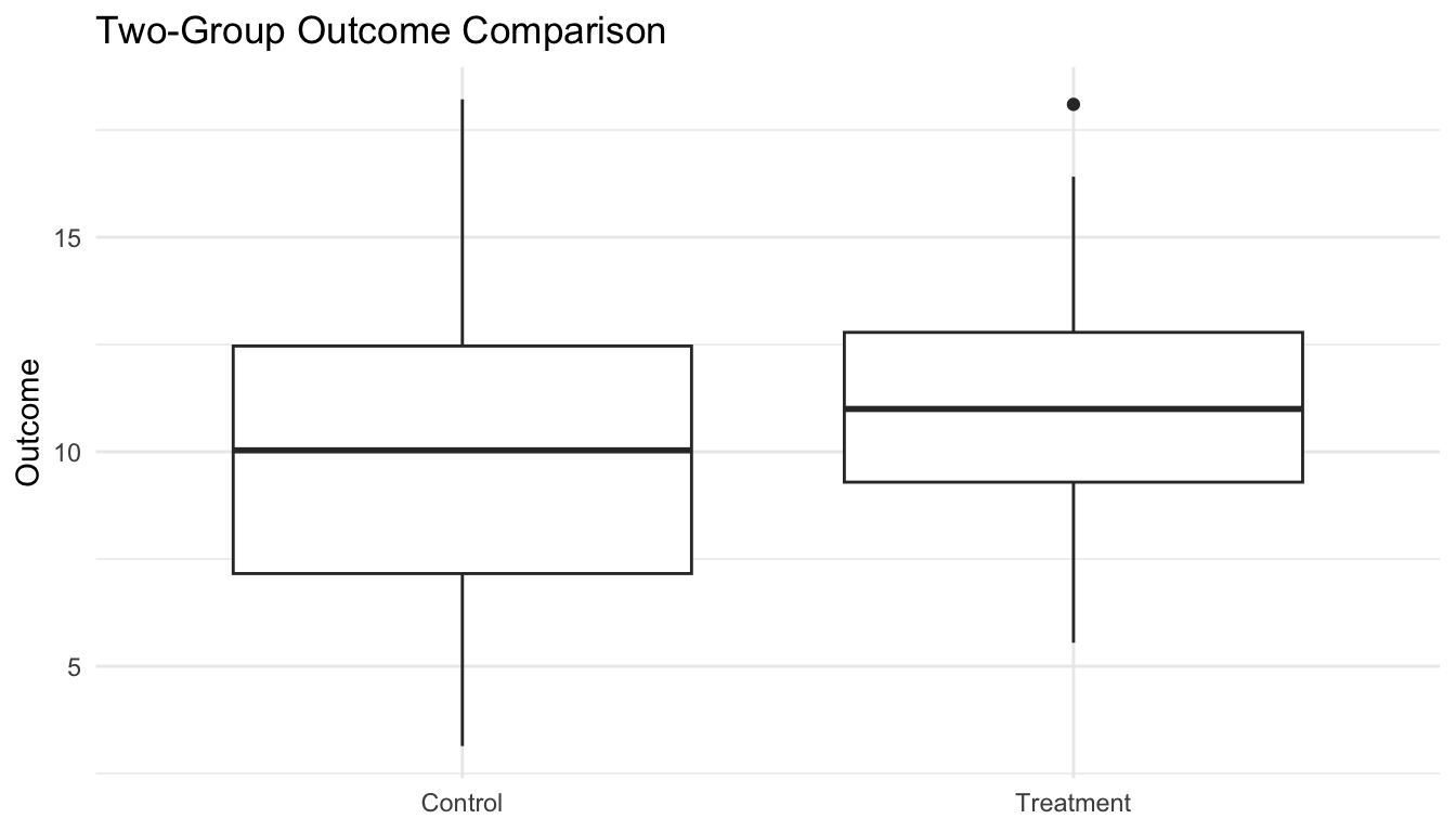
A t-test Is One of the Simplest Working Examples
A t-test compares means across groups.
We will simulate a small example with two groups.
library(dplyr)library(tibble)library(ggplot2)ttest_df <- tibble::tibble(group =rep(c("Control", "Treatment"), each =60),outcome =c(rnorm(60, mean =10, sd =3),rnorm(60, mean =11.2, sd =3) ))ttest_df |> dplyr::group_by(group) |> dplyr::summarise(n = dplyr::n(),mean =mean(outcome),sd =sd(outcome),.groups ="drop" )
# A tibble: 2 × 4
  group         n  mean    sd
  <chr>     <int> <dbl> <dbl>
1 Control      60  9.79  3.49
2 Treatment    60 11.1   2.78
Now conduct the t-test.
ttest_res <-t.test(outcome ~ group, data = ttest_df)ttest_res
    Welch Two Sample t-test

data:  outcome by group
t = -2.3153, df = 112.43, p-value = 0.02241
alternative hypothesis: true difference in means between group Control and group Treatment is not equal to 0
95 percent confidence interval:
 -2.4765335 -0.1925318
sample estimates:
  mean in group Control mean in group Treatment
               9.794092               11.128624
This output provides:
a test statistic,
degrees of freedom,
a p-value,
a confidence interval,
and group mean information.
That is already a reminder that the p-value should not be interpreted alone. The confidence interval often communicates much more.
Visualization Usually Improves Interpretation
Before and after formal testing, it helps to visualize the data.
That distinction matters enormously in both biostats and ML.
Confidence Intervals Often Tell a Better Story Than p-values Alone
Confidence intervals are often more informative than a binary significance label.
They communicate:
the estimated direction of effect,
the plausible range of values,
and the precision of the estimate.
For many readers, a confidence interval answers the practical question better than a p-value (Wasserstein and Lazar 2016).
The t-test output already included an interval for the difference in means. That interval often deserves more interpretive weight than the thresholded p-value.
In model evaluation, the same applies. Intervals around accuracy, AUC, calibration, or error rates often tell a more honest story than a single metric.
Power Determines What a Study Can Reasonably Detect
A non-significant result is hard to interpret without thinking about power.
     Two-sample t test power calculation

              n = 60
          delta = 1.2
             sd = 3
      sig.level = 0.05
          power = 0.5843645
    alternative = two.sided

NOTE: n is number in *each* group
This gives an approximate sense of whether the study is capable of detecting an effect of that size.
Low-power studies are not just inconvenient. They distort interpretation by making both positive and negative findings harder to trust.
Sample Size Planning Is an Ethical and Scientific Design Issue
Sample size is often treated as a technical afterthought, but it is really a design decision.
An underpowered study may:
miss meaningful effects,
waste resources,
and generate ambiguous conclusions.
An extremely large study may:
detect trivial effects,
overemphasize nominal significance,
and encourage overclaiming.
This is why sample size planning should be tied to:
plausible effect sizes,
decision relevance,
expected variability,
and the cost of Type I versus Type II errors.
In AI/ML experimentation, the same logic applies to online tests and validation studies.
Hypothesis Testing Still Matters in AI/ML
Some people frame hypothesis testing as an outdated concern compared with predictive modeling.
That is too simplistic.
Hypothesis testing still matters in AI/ML for problems such as:
A/B testing two models in production,
comparing feature sets,
evaluating whether a metric improved beyond noise,
testing subgroup differences in performance,
and screening whether observed improvements are likely to be sampling variation.
For example, if a new recommendation model appears 1 percent better than the old one, the right question is not only whether the metric increased, but whether the increase is stable, meaningful, and unlikely to reflect chance variation.
That is a testing problem.
Hypothesis Testing Can Also Be Misused in ML
At the same time, hypothesis testing can be badly misapplied in modern ML workflows.
Common mistakes include:
testing many features without multiplicity control,
declaring importance from univariate tests alone,
treating significance as predictive usefulness,
ignoring dependence across repeated experiments,
confusing validation noise with true improvement.
A feature can be statistically significant but practically useless for prediction. Conversely, a feature may not be individually significant in a small sample yet still contribute meaningfully in a multivariable predictive model.
This is one reason hypothesis testing should not be confused with model building.
Beyond p < 0.05 Means Thinking in Errors, Uncertainty, and Decisions
A mature use of hypothesis testing asks more than:
“Was the p-value below 0.05?”
It asks:
What was the null hypothesis?
Was the alternative scientifically meaningful?
What are the practical consequences of Type I and Type II errors?
How large is the effect?
How precise is the estimate?
Was the study adequately powered?
Would the result matter in deployment or decision-making?
This is especially important in high-stakes settings.
A small p-value does not decide whether a finding matters. People do.
A Small ML-Style Example: Comparing Model Accuracy
Suppose two models are evaluated on repeated resamples, producing two sets of accuracy estimates.
We can illustrate the temptation and the caution.
model_perf_df <- tibble::tibble(model =rep(c("Model A", "Model B"), each =40),accuracy =c(rnorm(40, mean =0.78, sd =0.03),rnorm(40, mean =0.80, sd =0.03) ))model_perf_df |> dplyr::group_by(model) |> dplyr::summarise(mean_accuracy =mean(accuracy),sd_accuracy =sd(accuracy),.groups ="drop" )
# A tibble: 2 × 3
  model   mean_accuracy sd_accuracy
  <chr>           <dbl>       <dbl>
1 Model A         0.783      0.0290
2 Model B         0.796      0.0230
t.test(accuracy ~ model, data = model_perf_df)
    Welch Two Sample t-test

data:  accuracy by model
t = -2.1781, df = 74.101, p-value = 0.03258
alternative hypothesis: true difference in means between group Model A and group Model B is not equal to 0
95 percent confidence interval:
 -0.02442401 -0.00108666
sample estimates:
mean in group Model A mean in group Model B
            0.7834150             0.7961704
This kind of comparison can be useful, but it also raises deeper questions:
are the resamples independent,
is the metric distribution well behaved,
is the effect practically meaningful,
and does significance translate into better operational performance?
In other words, testing is necessary, but not sufficient.
A Practical Checklist for Applied Work
Before reporting a hypothesis test, ask:
What exactly is the null hypothesis?
What result would count as practically meaningful?
What are the risks of Type I and Type II errors here?
Is the p-value being interpreted correctly?
What is the effect size?
What does the confidence interval say?
Was the analysis adequately powered?
Am I using significance as a shortcut for scientific or predictive relevance?
These questions greatly improve the quality of interpretation.
NoteWhere This Shows Up in AI/ML
A/B testing for clinical AI deployment — comparing model-assisted vs. standard-of-care decisions in a prospective trial — is formally a hypothesis test, and the same problems that plague p-values in research (underpowering, multiple comparisons, stopping at significance) appear in model evaluation: a study powered to detect a 5% reduction in missed sepsis diagnoses will almost never be powered for subgroup effects in the trauma population, yet subgroup failure is the most clinically dangerous failure mode. AI benchmark overfitting directly mirrors the replication crisis — models fine-tuned and re-evaluated on the same held-out set until they achieve a publishable AUC are doing implicit multiple comparisons without correction, inflating reported performance in exactly the way that produced a decade of irreproducible psychological findings.
Closing: Hypothesis Testing Still Matters, but Only If We Use It Well
Hypothesis testing remains useful because it gives structure to uncertainty.
It helps analysts ask whether observed differences are compatible with a null model. It formalizes false positive and false negative risk. It supports study planning through power and sample size logic.
But it becomes misleading when reduced to a ritual.
A p-value alone cannot tell us:
whether an effect matters,
whether a model is useful,
whether a feature improves prediction,
or whether a result should change practice.
Those judgments require effect sizes, intervals, design thinking, and domain context.
The real lesson of hypothesis testing in modern statistics and AI is not to abandon it, but to stop treating it like a binary oracle.
This post is part of the Trauma Registry Analytics Toolkit — a companion reference with hypothesis testing templates for multi-site registry data, effect size reporting, and power calculation scaffolds.
Casella, George, and Roger L. Berger. 2002. Statistical Inference. 2nd ed. Duxbury.
Wasserstein, Ronald L., and Nicole A. Lazar. 2016. “The ASA Statement on p-Values: Context, Process, and Purpose.”The American Statistician 70 (2): 129–33. https://doi.org/10.1080/00031305.2016.1154108.