Confidence Intervals: Your Shield Against Overconfident ML Models

Applied Statistics
Confidence Intervals
A practical guide to confidence intervals, coverage, bootstrap intervals, and uncertainty-aware interpretation for biostatistics and machine learning.
Published

October 15, 2023

Modified

June 9, 2026

Executive Summary

Point estimates are easy to report and easy to overtrust.

A mean can be written as a single number. A proportion can be written as a percentage. A model performance metric can be summarized with one statistic.

But none of those numbers are exact. They are estimates built from finite data.

Confidence intervals provide a disciplined way to express that uncertainty (Casella and Berger 2002; Wasserman 2004).

Rather than saying only:

  • the mean is 12.4,
  • the response rate is 68%,
  • the model accuracy is 0.81,

confidence intervals say:

  • how precise the estimate is,
  • how much sampling variation is plausible,
  • and how cautious we should be when drawing conclusions.

This matters in both biostatistics and machine learning.

In biostatistics, confidence intervals help with:

  • treatment effect interpretation,
  • outcome rate estimation,
  • and study reporting.

In AI/ML, they help with:

  • uncertainty around model performance,
  • prediction intervals and uncertainty bounds,
  • calibration of claims,
  • and avoiding overconfident model communication.

A point estimate tells you what you saw. A confidence interval reminds you what you do not know with certainty.


Confidence Intervals Exist Because Estimates Are Noisy

Any estimate based on a sample is subject to variation.

If we drew a different sample from the same population, we would likely get a slightly different mean, proportion, regression slope, or performance metric.

That is not a flaw in statistics. It is the basic reality of learning from incomplete information.

Confidence intervals give us a structured way to quantify this uncertainty.

They do not eliminate noise. They make it visible.

This is one reason confidence intervals are so useful in applied work.

A result without uncertainty is often more persuasive-looking than it deserves to be.


What a Confidence Interval Actually Means

A confidence interval is commonly misunderstood.

A 95% confidence interval does not mean:

there is a 95% probability that the true parameter lies inside this particular interval.

Under the classical interpretation, the true parameter is fixed and the interval is random.

A 95% confidence interval means that:

if we repeated the sampling process many times and constructed intervals the same way each time, about 95% of those intervals would contain the true parameter.

This is a statement about the long-run behavior of the procedure.

That may feel subtle, but it matters.

Confidence intervals are best understood as properties of an estimation method, not as literal posterior probabilities.


Coverage Probability Is the Core Idea

The key technical idea behind confidence intervals is coverage.

Coverage probability is the proportion of repeated intervals that successfully contain the true parameter (Casella and Berger 2002).

For a nominal 95% confidence interval procedure, we hope the true long-run coverage is close to 0.95.

That does not mean every single interval will work. Some will miss.

This is why confidence intervals are not guarantees. They are uncertainty procedures with known operating characteristics, at least under assumptions.

Coverage is one of the most important concepts to understand if we want to interpret intervals honestly.


Parametric Confidence Intervals Depend on Distributional Assumptions

A parametric confidence interval relies on an assumed probability model.

For example:

  • a normal-theory interval for a mean,
  • a Wald-style interval for a proportion,
  • a t-based interval when the variance is estimated from the data.

These intervals are often efficient and familiar. But their performance depends on assumptions being at least reasonably appropriate.

This is why applied analysts should understand not only how to compute intervals, but also what assumptions support them.


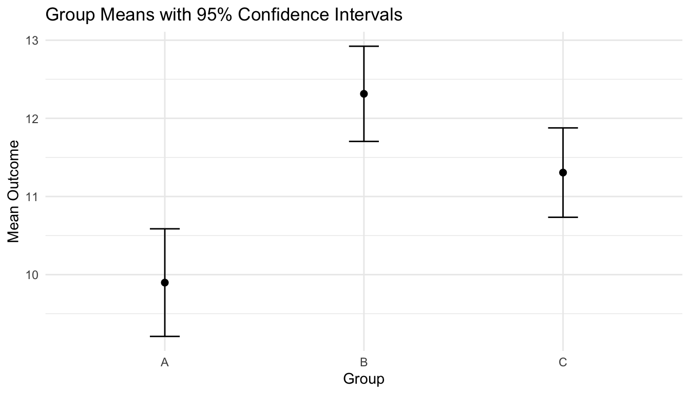
A Parametric Confidence Interval for a Mean

We begin with a simple example: estimating a population mean.

library(dplyr)
library(tibble)
library(ggplot2)

mean_df <- tibble::tibble(
  outcome = rnorm(80, mean = 12, sd = 4)
)

mean_df |>
  dplyr::summarise(
    n = dplyr::n(),
    sample_mean = mean(outcome),
    sample_sd = sd(outcome)
  )
# A tibble: 1 × 3
      n sample_mean sample_sd
  <int>       <dbl>     <dbl>
1    80        12.1      4.41

Now compute a classical t-based confidence interval for the mean.

t.test(mean_df$outcome)$conf.int
[1] 11.07843 13.04150
attr(,"conf.level")
[1] 0.95

This is a parametric interval because it relies on the t distribution and the usual assumptions behind it.

It is often a good default when the data are roughly symmetric or the sample size is moderate.


A Parametric Confidence Interval for a Proportion

Confidence intervals are also common for proportions.

Suppose we observe a binary outcome such as response/no response.

prop_df <- tibble::tibble(
  response = rbinom(120, size = 1, prob = 0.68)
)

prop_df |>
  dplyr::summarise(
    n = dplyr::n(),
    successes = sum(response),
    p_hat = mean(response)
  )
# A tibble: 1 × 3
      n successes p_hat
  <int>     <int> <dbl>
1   120        79 0.658

A simple way to obtain a proportion interval in R is prop.test().

prop.test(sum(prop_df$response), nrow(prop_df), correct = FALSE)$conf.int
[1] 0.5697483 0.7370956
attr(,"conf.level")
[1] 0.95

This gives an approximate confidence interval for the response probability.

Intervals for proportions are especially important because raw percentages can look more certain than they really are, particularly in small samples.


Non-Parametric Confidence Intervals Reduce Dependence on Strong Assumptions

A non-parametric confidence interval avoids or reduces reliance on a strict parametric distributional model.

One of the most practical tools here is the bootstrap.

The bootstrap repeatedly resamples from the observed dataset and approximates the sampling distribution of a statistic empirically (Efron and Tibshirani 1993).

This is useful when:

  • analytic formulas are inconvenient,
  • assumptions are uncertain,
  • or the statistic is more complicated than a simple mean.

Non-parametric does not mean assumption-free. But it often means assumption-light.


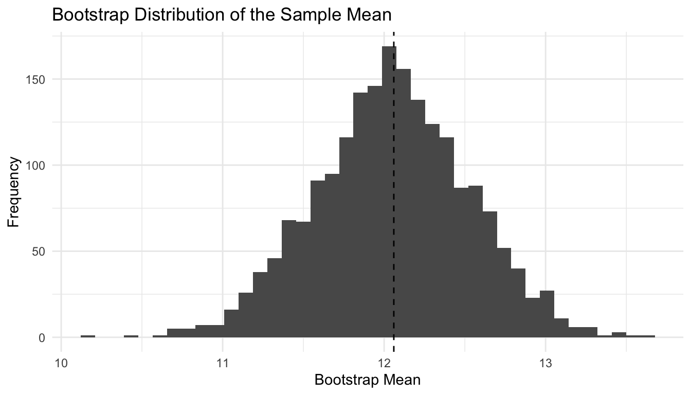
A Bootstrap Confidence Interval for a Mean

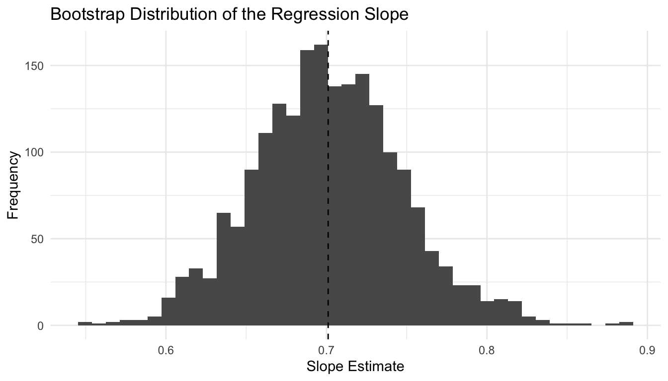
We can construct a bootstrap interval for the mean by repeatedly resampling the observed data with replacement.

boot_mean_df <- tibble::tibble(
  rep = 1:2000,
  boot_mean = replicate(
    2000,
    {
      boot_sample <- mean_df |>
        dplyr::slice_sample(n = nrow(mean_df), replace = TRUE)
      mean(boot_sample$outcome)
    }
  )
)

boot_mean_df |>
  dplyr::summarise(
    mean_boot = mean(boot_mean),
    ci_lower = quantile(boot_mean, 0.025),
    ci_upper = quantile(boot_mean, 0.975)
  )
# A tibble: 1 × 3
  mean_boot ci_lower ci_upper
      <dbl>    <dbl>    <dbl>
1      12.1     11.1     13.0

And visualize the bootstrap distribution.

ggplot2::ggplot(boot_mean_df, ggplot2::aes(x = boot_mean)) +
  ggplot2::geom_histogram(bins = 40) +
  ggplot2::geom_vline(xintercept = mean(mean_df$outcome), linetype = 2) +
  ggplot2::labs(
    title = "Bootstrap Distribution of the Sample Mean",
    x = "Bootstrap Mean",
    y = "Frequency"
  ) +
  ggplot2::theme_minimal()

This gives a direct empirical view of how the mean might vary across repeated samples.


Bootstrap Intervals Are Also Useful for Proportions

The bootstrap can be used for proportions just as easily.

boot_prop_df <- tibble::tibble(
  rep = 1:2000,
  boot_prop = replicate(
    2000,
    {
      boot_sample <- prop_df |>
        dplyr::slice_sample(n = nrow(prop_df), replace = TRUE)
      mean(boot_sample$response)
    }
  )
)

boot_prop_df |>
  dplyr::summarise(
    mean_boot = mean(boot_prop),
    ci_lower = quantile(boot_prop, 0.025),
    ci_upper = quantile(boot_prop, 0.975)
  )
# A tibble: 1 × 3
  mean_boot ci_lower ci_upper
      <dbl>    <dbl>    <dbl>
1     0.659    0.575    0.742

This is especially helpful when sample sizes are smaller or when the analyst wants a more simulation-based interval rather than a formula-based one.


Confidence Intervals Are Often Better Communicators Than Hypothesis Tests

Confidence intervals and hypothesis tests are closely related, but intervals often communicate more.

A p-value mainly addresses whether the data are compatible with a null value. A confidence interval also shows:

  • direction,
  • magnitude,
  • and precision.

For decision-making, those are often more useful.

For example, a narrow interval around a small effect tells a different story than a wide interval spanning both meaningful benefit and possible harm.

That is why many analysts prefer to foreground intervals rather than binary significance labels (Wasserstein and Lazar 2016).


Visualizing Confidence Intervals Makes Uncertainty Harder to Ignore

One of the best ways to teach and communicate confidence intervals is with error bars.

Below is a simple example comparing group means with intervals.

group_df <- tibble::tibble(
  group = rep(c("A", "B", "C"), each = 50),
  outcome = c(
    rnorm(50, mean = 10, sd = 2),
    rnorm(50, mean = 12, sd = 2.5),
    rnorm(50, mean = 11, sd = 2.2)
  )
)

group_ci_df <- group_df |>
  dplyr::group_by(group) |>
  dplyr::summarise(
    n = dplyr::n(),
    mean = mean(outcome),
    sd = sd(outcome),
    se = sd / sqrt(n),
    lower = mean + qt(0.025, df = n - 1) * se,
    upper = mean + qt(0.975, df = n - 1) * se,
    .groups = "drop"
  )

group_ci_df
# A tibble: 3 × 7
  group     n  mean    sd    se lower upper
  <chr> <int> <dbl> <dbl> <dbl> <dbl> <dbl>
1 A        50  9.90  2.42 0.343  9.21  10.6
2 B        50 12.3   2.14 0.303 11.7   12.9
3 C        50 11.3   2.01 0.285 10.7   11.9
ggplot2::ggplot(group_ci_df, ggplot2::aes(x = group, y = mean)) +
  ggplot2::geom_point(size = 2) +
  ggplot2::geom_errorbar(ggplot2::aes(ymin = lower, ymax = upper), width = 0.15) +
  ggplot2::labs(
    title = "Group Means with 95% Confidence Intervals",
    x = "Group",
    y = "Mean Outcome"
  ) +
  ggplot2::theme_minimal()

Plots like this are helpful because they push readers beyond point estimates and toward uncertainty-aware interpretation.


Confidence Intervals Matter in AI/ML Because Predictions Without Uncertainty Can Mislead

Many modern AI systems produce predictions that look precise.

But precision in formatting is not the same as certainty in inference.

Confidence intervals matter in AI/ML for tasks such as:

  • uncertainty around model performance metrics,
  • interval estimates for calibration or error rates,
  • uncertainty in regression coefficients,
  • bootstrap intervals for feature effects,
  • prediction intervals,
  • and uncertainty-aware deployment.

This is especially important in high-stakes settings.

A model that outputs a confident-looking number without uncertainty can easily encourage overtrust.

That is one reason interval thinking is central to interpretable and responsible AI.


Confidence Intervals and Prediction Intervals Are Not the Same

This distinction is often overlooked.

A confidence interval quantifies uncertainty about a parameter, such as a mean.

A prediction interval quantifies uncertainty about a future observation.

Prediction intervals are usually wider because they must account for both:

  • uncertainty in the estimated mean structure,
  • and individual-level variability around that structure.

This matters in ML, where people often want uncertainty around predictions, not just uncertainty around average parameters.

Confidence intervals are useful, but they are not always the interval the user actually needs.


A Bootstrap Confidence Interval for a Regression Slope

To connect intervals to modeling, we can bootstrap a regression coefficient.

reg_df <- tibble::tibble(
  x = rnorm(150, mean = 50, sd = 10)
) |>
  dplyr::mutate(
    y = 5 + 0.7 * x + rnorm(150, mean = 0, sd = 6)
  )

fit_lm <- lm(y ~ x, data = reg_df)
summary(fit_lm)$coefficients
             Estimate Std. Error t value     Pr(>|t|)
(Intercept) 5.3384643 2.71705200  1.9648 5.131000e-02
x           0.7010675 0.05295312 13.2394 6.869901e-27

Now bootstrap the slope.

boot_slope_df <- tibble::tibble(
  rep = 1:2000,
  slope = replicate(
    2000,
    {
      boot_sample <- reg_df |>
        dplyr::slice_sample(n = nrow(reg_df), replace = TRUE)
      coef(lm(y ~ x, data = boot_sample))[["x"]]
    }
  )
)

boot_slope_df |>
  dplyr::summarise(
    mean_slope = mean(slope),
    ci_lower = quantile(slope, 0.025),
    ci_upper = quantile(slope, 0.975)
  )
# A tibble: 1 × 3
  mean_slope ci_lower ci_upper
       <dbl>    <dbl>    <dbl>
1      0.701    0.612    0.800

And visualize it.

ggplot2::ggplot(boot_slope_df, ggplot2::aes(x = slope)) +
  ggplot2::geom_histogram(bins = 40) +
  ggplot2::geom_vline(xintercept = coef(fit_lm)[["x"]], linetype = 2) +
  ggplot2::labs(
    title = "Bootstrap Distribution of the Regression Slope",
    x = "Slope Estimate",
    y = "Frequency"
  ) +
  ggplot2::theme_minimal()

This is often an intuitive way to show uncertainty in model parameters without depending exclusively on asymptotic formulas.


Confidence Intervals Can Be Misused Too

Confidence intervals are often better than single p-values, but they can still be misread.

Common mistakes include:

  • treating them as probability statements about a fixed interval,
  • focusing only on whether the null value is included,
  • ignoring assumptions behind the interval,
  • mistaking narrowness for correctness,
  • forgetting that biased data can produce misleadingly precise intervals.

An interval can be narrow and still be wrong if the design, sampling, or measurement process is flawed.

So intervals improve communication, but they do not rescue bad data.


A Practical Checklist for Applied Work

Before reporting a confidence interval, ask:

  • What parameter does this interval refer to?
  • Is it parametric or non-parametric?
  • What assumptions support it?
  • Is the interval estimating a mean, a proportion, a regression effect, or a future prediction?
  • Does the interval show uncertainty clearly enough for the real decision?
  • Am I confusing confidence intervals with prediction intervals?
  • Does the width of the interval meaningfully affect interpretation?

These questions improve both rigor and clarity.

NoteWhere This Shows Up in AI/ML

Prediction intervals — not confidence intervals — are the correct output for individual-level clinical AI decisions: a model predicting 72-hour mortality for a specific trauma patient should report a prediction interval communicating the range of plausible outcomes for that individual, not a confidence interval around the mean prediction across similar patients. The FDA’s guidance on AI/ML-based medical devices now treats prediction interval width as a deployment readiness criterion, recognizing that a model with a point AUC of 0.84 but 95% prediction intervals spanning 0.3–0.95 across individual patients offers false precision that can mislead clinicians into overconfident action at the bedside.


Closing: Confidence Intervals Protect Against False Precision

Confidence intervals are one of the most useful tools in applied statistics because they resist the false certainty of point estimates.

They remind us that every estimate is conditional on finite data, variability, and assumptions.

That is true in biostatistics. It is equally true in AI and machine learning.

Confidence intervals help us:

  • communicate uncertainty,
  • compare estimates more honestly,
  • understand precision,
  • and resist overconfident claims from models or analysts.

Confidence intervals are not just a technical add-on. They are one of the simplest ways to force humility back into quantitative analysis.


Tip📚 Go Deeper: Prediction Modeling Toolkit

This post is part of the Prediction Modeling Toolkit — a companion reference with interval estimation templates, bootstrap CI code, and reporting language for clinical prediction uncertainty.

→ Open the Prediction Modeling Toolkit


Series Callout

Note

This post is part of a broader Applied Statistics for AI and Clinical Decision-Making Series:

  • Probability fundamentals for machine learning
  • Random variables and expectation
  • Common probability distributions
  • Central Limit Theorem
  • Law of Large Numbers
  • Sampling methods for Biostats and ML
  • Hypothesis testing in the age of AI
  • Confidence intervals
  • Maximum likelihood estimation
  • Bayesian inference
  • Linear regression
  • Logistic regression
  • Generalized linear models
  • Analysis of variance
  • Principal component analysis
  • Cluster analysis
  • Time series analysis
  • Survival analysis
  • Non-parametric methods
  • Bias-variance tradeoff
  • Regularization
  • Cross-validation
  • Information theory
  • Optimization techniques
  • Linear algebra basics
  • Calculus for ML
  • Monte Carlo methods
  • Dimensionality curse and reduction techniques
  • Model evaluation metrics
  • Ensemble methods

References

Casella, George, and Roger L. Berger. 2002. Statistical Inference. 2nd ed. Duxbury.
Efron, Bradley, and Robert J. Tibshirani. 1993. An Introduction to the Bootstrap. Chapman & Hall. https://doi.org/10.1201/9780429246593.
Wasserman, Larry. 2004. All of Statistics: A Concise Course in Statistical Inference. Springer.
Wasserstein, Ronald L., and Nicole A. Lazar. 2016. “The ASA Statement on p-Values: Context, Process, and Purpose.” The American Statistician 70 (2): 129–33. https://doi.org/10.1080/00031305.2016.1154108.