Maximum Likelihood Estimation Unlocked: Training AI Models Like a Statistician

Applied Statistics
Maximum Likelihood Estimation
An applied introduction to likelihood, log-likelihood, maximum likelihood estimation, and numerical optimization for AI and clinical modeling.
Published

November 15, 2023

Modified

June 9, 2026

Executive Summary

Maximum likelihood estimation is one of the central ideas connecting classical statistics and modern machine learning (Fisher 1922; Casella and Berger 2002; Murphy 2012).

At a high level, MLE asks a simple question:

Which parameter values make the observed data most plausible under the model?

That question is both mathematically elegant and practically powerful.

It drives estimation in many familiar statistical models, and it also sits underneath much of modern AI/ML, including:

  • logistic regression,
  • probabilistic classifiers,
  • latent-variable models,
  • and the EM algorithm used in unsupervised learning.

MLE matters because it turns model fitting into an optimization problem.

Instead of guessing parameters, we define a probability model for the data and then choose the parameter values that maximize the likelihood of what we actually observed.

This post introduces:

  • the intuition behind likelihood,
  • MLE for common distributions,
  • custom likelihood coding in R,
  • numerical optimization,
  • and comparison with method of moments.

MLE is one of the clearest examples of statistics and machine learning speaking the same language: model the data-generating process, write the objective function, and optimize.


Likelihood Turns Model Fitting into an Optimization Problem

In probability, we often think forward:

  • given a parameter value,
  • what is the probability of the data?

Likelihood reverses the emphasis.

In likelihood-based inference, the data are treated as fixed and the parameter is treated as unknown.

We ask:

for the observed data, which parameter values make them most plausible?

This shift is subtle but fundamental.

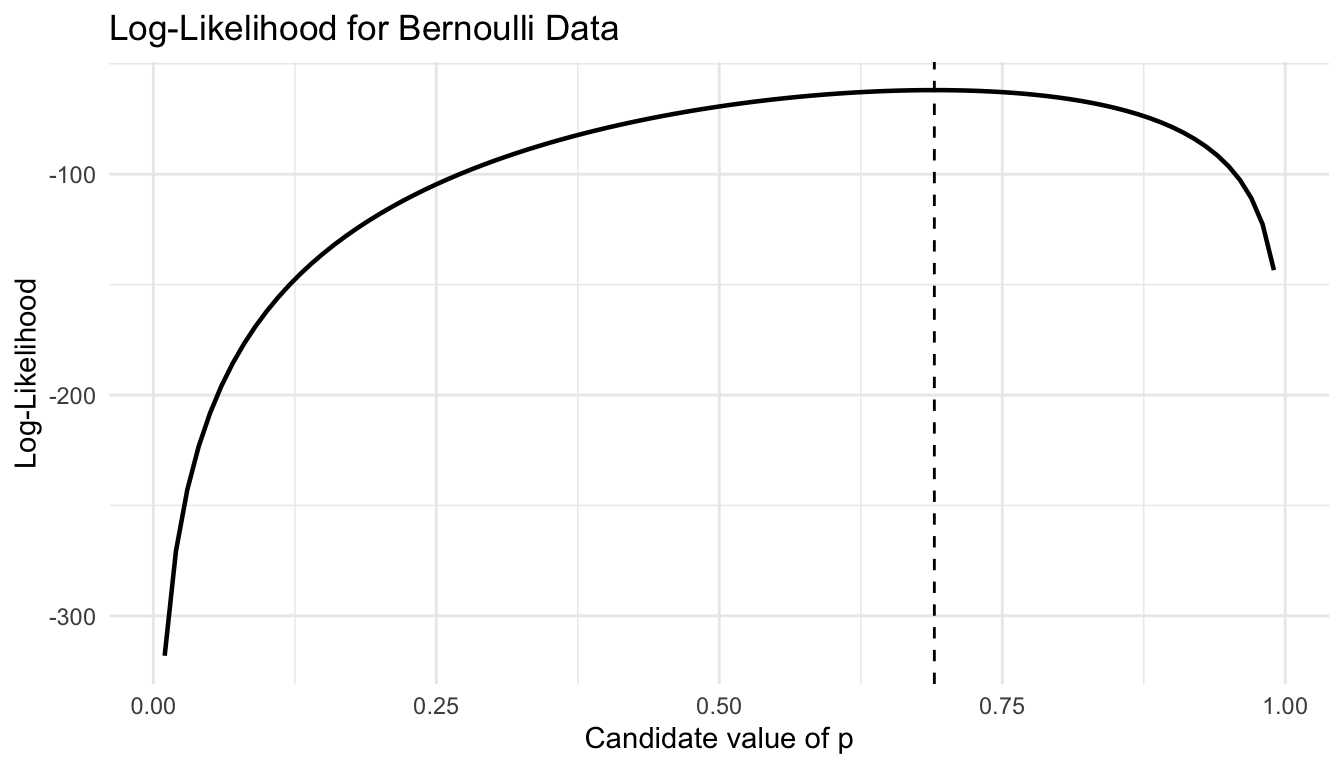
A likelihood function is not a probability distribution over the parameter in the classical sense. It is a function of the parameter, indexed by the observed data.

That is why MLE is so powerful.

It turns estimation into a problem of finding the parameter value that maximizes a function (Fisher 1922; DeGroot and Schervish 2012).


The Likelihood Function Is Built from the Data Model

Suppose \(X_1, X_2, \dots, X_n\) are independent observations from a model with parameter \(\theta\).

The likelihood is:

\[ L(\theta \mid x_1, \dots, x_n) = \prod_{i=1}^n f(x_i \mid \theta) \]

where \(f(\cdot)\) is the probability mass function or density function.

In practice, we often work with the log-likelihood:

\[ \ell(\theta) = \log L(\theta) \]

This is convenient because products turn into sums:

\[ \ell(\theta) = \sum_{i=1}^n \log f(x_i \mid \theta) \]

The log-likelihood is easier to compute, easier to differentiate, and numerically more stable.

This is the version most analysts and machine learning practitioners actually optimize.


The Core MLE Idea Is Simple Even If the Math Varies

The maximum likelihood estimator is the parameter value:

\[ \hat{\theta}_{\mathrm{MLE}} = \arg\max_{\theta} L(\theta) \]

or equivalently,

\[ \hat{\theta}_{\mathrm{MLE}} = \arg\max_{\theta} \ell(\theta) \]

Conceptually, that means:

  • write down the data model,
  • write down the likelihood,
  • simplify if possible,
  • maximize with respect to the unknown parameter.

Sometimes this yields a closed-form solution. Sometimes it requires numerical optimization.

Either way, the underlying logic is the same.


A Bernoulli Example Makes the Idea Concrete

Suppose we observe binary data, such as success/failure outcomes.

If \(X_i \sim \text{Bernoulli}(p)\), then:

\[ P(X_i = x_i) = p^{x_i}(1-p)^{1-x_i} \]

For an independent sample, the likelihood is:

\[ L(p) = \prod_{i=1}^n p^{x_i}(1-p)^{1-x_i} \]

This simplifies to:

\[ L(p) = p^{\sum x_i}(1-p)^{n-\sum x_i} \]

The MLE turns out to be the sample proportion:

\[ \hat{p}_{MLE} = \bar{x} \]

We can verify this with a simple example.

library(dplyr)
library(tibble)
library(ggplot2)

bern_df <- tibble::tibble(
  x = rbinom(100, size = 1, prob = 0.70)
)

bern_df |>
  dplyr::summarise(
    n = dplyr::n(),
    successes = sum(x),
    p_hat = mean(x)
  )
# A tibble: 1 × 3
      n successes p_hat
  <int>     <int> <dbl>
1   100        69  0.69

For Bernoulli data, the sample mean and sample proportion are the same quantity.

This is one of the simplest MLE results, but it is already very important.

It connects directly to logistic regression and binary classification.


Visualizing the Likelihood Helps Demystify It

A nice way to understand likelihood is to calculate it across a grid of candidate parameter values.

p_grid <- seq(0.01, 0.99, by = 0.01)

loglik_bern <- function(p, x) {
  sum(dbinom(x, size = 1, prob = p, log = TRUE))
}

bern_like_df <- tibble::tibble(
  p = p_grid,
  loglik = purrr::map_dbl(p_grid, ~ loglik_bern(.x, bern_df$x))
)

ggplot2::ggplot(bern_like_df, ggplot2::aes(x = p, y = loglik)) +
  ggplot2::geom_line(linewidth = 0.8) +
  ggplot2::geom_vline(xintercept = mean(bern_df$x), linetype = 2) +
  ggplot2::labs(
    title = "Log-Likelihood for Bernoulli Data",
    x = "Candidate value of p",
    y = "Log-Likelihood"
  ) +
  ggplot2::theme_minimal()

The peak of this curve is the maximum likelihood estimate.

This kind of plot is useful because it shows that MLE is not magic. It is just optimization over a model-based objective function.


A Normal Example Shows a Familiar Closed-Form Result

Suppose the data follow a normal distribution:

\[ X_i \sim N(\mu, \sigma^2) \]

If \(\sigma^2\) is known, the MLE for \(\mu\) is the sample mean.

If both \(\mu\) and \(\sigma^2\) are unknown, the MLEs are:

\[ \hat{\mu}_{MLE} = \bar{x} \]

\[ \hat{\sigma}^2_{MLE} = \frac{1}{n} \sum_{i=1}^n (x_i - \bar{x})^2 \]

That variance formula is slightly different from the unbiased sample variance, which divides by (n-1).

Let us demonstrate.

norm_df <- tibble::tibble(
  x = rnorm(150, mean = 12, sd = 3)
)

mu_hat_mle <- mean(norm_df$x)
sigma2_hat_mle <- mean((norm_df$x - mu_hat_mle)^2)

tibble::tibble(
  mu_hat_mle = mu_hat_mle,
  sigma_hat_mle = sqrt(sigma2_hat_mle),
  sd_r = sd(norm_df$x)
)
# A tibble: 1 × 3
  mu_hat_mle sigma_hat_mle  sd_r
       <dbl>         <dbl> <dbl>
1       11.7          2.96  2.97

This is a useful reminder that MLE and unbiasedness are not identical goals (Casella and Berger 2002).

MLE prioritizes likelihood maximization, not necessarily unbiasedness in small samples.


Method of Moments Solves a Different Problem

The method of moments is another classical estimation strategy.

Instead of maximizing likelihood, it matches sample moments to theoretical moments.

For example:

  • sample mean matched to theoretical mean,
  • sample variance matched to theoretical variance.

In some simple models, method of moments and MLE coincide. In others, they differ.

This makes for a useful comparison.

MLE asks:

which parameter values make the data most plausible?

Method of moments asks:

which parameter values reproduce key summary features of the data?

Both can be useful, but MLE tends to have stronger general theoretical and practical connections to modern model fitting.


A Poisson Example Compares MLE and Method of Moments

For Poisson data with parameter \(\lambda\),

\[ P(X = x) = \frac{e^{-\lambda}\lambda^x}{x!} \]

Both the mean and variance equal \(\lambda\).

That means the method of moments estimator and the MLE both equal the sample mean.

pois_df <- tibble::tibble(
  x = rpois(200, lambda = 4.5)
)

lambda_hat_mle <- mean(pois_df$x)
lambda_hat_mom <- mean(pois_df$x)

tibble::tibble(
  mle = lambda_hat_mle,
  method_of_moments = lambda_hat_mom
)
# A tibble: 1 × 2
    mle method_of_moments
  <dbl>             <dbl>
1   4.3               4.3

This is a nice example where the two approaches agree.

But that agreement is not universal.


Sometimes We Need Numerical Optimization Instead of Algebra

Many models do not yield closed-form MLEs.

In those cases, we use numerical optimization.

This is a major reason MLE matters so much for AI/ML (Murphy 2012; Hastie et al. 2009).

Once the objective function is written down, the fitting problem becomes computational.

We can illustrate this with a custom normal log-likelihood.

neg_loglik_normal <- function(par, x) {
  mu <- par[1]
  sigma <- par[2]
  
  if (sigma <= 0) {
    return(Inf)
  }
  
  -sum(dnorm(x, mean = mu, sd = sigma, log = TRUE))
}

optim_res <- optim(
  par = c(mean(norm_df$x), sd(norm_df$x)),
  fn = neg_loglik_normal,
  x = norm_df$x
)

optim_res$par
[1] 11.719991  2.965101

This gives the numerically optimized MLEs for the normal mean and standard deviation.

They should be very close to the analytic results we computed earlier.

tibble::tibble(
  parameter = c("mu", "sigma"),
  analytic = c(mu_hat_mle, sqrt(sigma2_hat_mle)),
  numeric = optim_res$par
)
# A tibble: 2 × 3
  parameter analytic numeric
  <chr>        <dbl>   <dbl>
1 mu           11.7    11.7 
2 sigma         2.96    2.97

This is the same basic pattern used in many more complex models.


Writing a Custom Likelihood Is One of the Best Ways to Learn MLE

A very effective way to understand MLE is to code the likelihood directly.

Let us return to the Poisson example and write a custom log-likelihood function.

neg_loglik_poisson <- function(lambda, x) {
  if (lambda <= 0) {
    return(Inf)
  }
  
  -sum(dpois(x, lambda = lambda, log = TRUE))
}

opt_pois <- optimize(
  f = neg_loglik_poisson,
  interval = c(0.001, 20),
  x = pois_df$x
)

tibble::tibble(
  mle_by_optimization = opt_pois$minimum,
  mle_by_formula = mean(pois_df$x)
)
# A tibble: 1 × 2
  mle_by_optimization mle_by_formula
                <dbl>          <dbl>
1                4.30            4.3

This is a good bridge to more advanced models.

Once you can write a likelihood, you can often estimate the model.

That is a powerful skill for both statisticians and machine learning practitioners (Murphy 2012).


Logistic Regression Is an MLE Problem

One reason MLE is so central to ML is that many common learning algorithms are maximum likelihood procedures in disguise.

For logistic regression, the outcome is binary and the model assumes:

\[ P(Y_i = 1 \mid X_i) = \pi_i \]

with

\[ \log \left( \frac{\pi_i}{1-\pi_i} \right) = \beta_0 + \beta_1 X_i \]

The parameters are estimated by maximizing the Bernoulli likelihood across all observations.

That means logistic regression is fundamentally an MLE problem.

The same general logic extends to:

  • multinomial regression,
  • Poisson regression,
  • Gaussian models,
  • and many latent-variable models.

In other words, MLE is not a niche statistical trick. It is one of the engines of predictive modeling.


MLE Connects Naturally to Loss Functions in ML

Machine learning practitioners often think in terms of minimizing loss, not maximizing likelihood.

But the two are often equivalent.

For many probabilistic models:

  • maximizing the log-likelihood
  • is the same as minimizing the negative log-likelihood

This is why so many ML training objectives look like:

  • cross-entropy loss,
  • log loss,
  • negative log-likelihood,
  • deviance.

They are all variations on the same principle.

That is one of the reasons MLE is such an important bridge between classical inference and modern ML training.


The EM Algorithm Extends MLE to Incomplete or Latent Data Settings

MLE becomes more complicated when the data are incomplete or when the model contains latent variables.

That is where the Expectation-Maximization (EM) algorithm becomes useful.

The EM idea is:

  • E-step: compute expected sufficient quantities given current parameter values,
  • M-step: maximize the expected complete-data log-likelihood.

This appears in settings such as:

  • Gaussian mixture models,
  • latent class models,
  • missing-data problems,
  • clustering and unsupervised learning.

You do not need the full EM derivation to appreciate the connection: it is still an MLE problem, but solved iteratively when direct optimization is harder.


MLE Has Strengths, but It Also Has Assumptions

MLE is powerful, but it is not assumption-free.

Its quality depends on:

  • whether the model family is sensible,
  • whether observations are appropriately modeled,
  • whether independence assumptions are reasonable,
  • whether the optimizer behaves well,
  • and whether the likelihood surface is well behaved.

A beautifully optimized likelihood under the wrong model can still produce misleading answers.

This is an important lesson in both biostatistics and AI.

Optimization is not the same as truth. It is only as good as the model being optimized.


A Small Regression-Style Example Using Negative Log-Likelihood

To make the ML connection even more explicit, here is a simple binary outcome example with a custom Bernoulli negative log-likelihood for an intercept-only model.

y_bin <- rbinom(200, size = 1, prob = 0.65)

neg_loglik_intercept_only <- function(beta0, y) {
  p <- 1 / (1 + exp(-beta0))
  
  if (any(p <= 0 | p >= 1)) {
    return(Inf)
  }
  
  -sum(dbinom(y, size = 1, prob = p, log = TRUE))
}

opt_intercept <- optimize(
  f = neg_loglik_intercept_only,
  interval = c(-10, 10),
  y = y_bin
)

beta0_hat <- opt_intercept$minimum
p_hat <- 1 / (1 + exp(-beta0_hat))

tibble::tibble(
  estimated_intercept = beta0_hat,
  estimated_probability = p_hat,
  sample_proportion = mean(y_bin)
)
# A tibble: 1 × 3
  estimated_intercept estimated_probability sample_proportion
                <dbl>                 <dbl>             <dbl>
1               0.641                 0.655             0.655

This illustrates an important point:

even a simple classifier can be understood as a likelihood optimization problem.

That is the core MLE idea appearing in ML language.


A Practical Checklist for Applied Work

Before using or reporting an MLE-based fit, ask:

  • What probability model am I assuming for the data?
  • What is the likelihood function?
  • Do I have a closed-form estimator or do I need optimization?
  • Does the estimate make sense relative to the data?
  • How sensitive is the result to assumptions or starting values?
  • Would method of moments give a similar answer?
  • Am I optimizing a sensible model, or only optimizing efficiently?

These questions usually improve both understanding and interpretation.

NoteWhere This Shows Up in AI/ML

Cross-entropy loss — the objective function used to train virtually every neural network classifier, including clinical NLP models that extract injury severity from trauma notes and sepsis prediction models that consume EHR time series — is the negative log-likelihood under a Bernoulli or categorical distribution, making MLE the literal mechanism by which these models learn from data. When the training data is class-imbalanced (as it always is in trauma: severe TBI is rare even in the DoDTR), the MLE objective is dominated by the majority class and the resulting model is optimized to predict “no severe outcome” almost always — a failure that emerges directly from what MLE maximizes and can only be fixed by modifying the likelihood (weighted loss, focal loss) or the sampling strategy.


Closing: MLE Is One of the Main Languages Shared by Statistics and ML

Maximum likelihood estimation is powerful because it gives a general recipe for learning from data.

It says:

  • define a probability model,
  • quantify how plausible the observed data are under candidate parameters,
  • and choose the parameter values that maximize that plausibility.

That logic is elegant enough for theory and practical enough for real model training.

It appears in:

  • Bernoulli models,
  • normal models,
  • logistic regression,
  • count models,
  • and iterative procedures like EM.

MLE matters because it turns model fitting into a coherent, general-purpose optimization problem — one that sits at the heart of both statistical inference and machine learning.


Tip📚 Go Deeper: Bayesian Workflow Toolkit

This post is part of the Bayesian Workflow Toolkit — a companion reference with likelihood specification templates, MLE-to-Bayesian bridge examples, and numerical optimization scaffolds.

→ Open the Bayesian Workflow Toolkit


Series Callout

Note

This post is part of a broader Applied Statistics for AI and Clinical Decision-Making Series:

  • Probability fundamentals for machine learning
  • Random variables and expectation
  • Common probability distributions
  • Central Limit Theorem
  • Law of Large Numbers
  • Sampling methods for Biostats and ML
  • Hypothesis testing in the age of AI
  • Confidence intervals
  • Maximum likelihood estimation
  • Bayesian inference
  • Linear regression
  • Logistic regression
  • Generalized linear models
  • Analysis of variance
  • Principal component analysis
  • Cluster analysis
  • Time series analysis
  • Survival analysis
  • Non-parametric methods
  • Bias-variance tradeoff
  • Regularization
  • Cross-validation
  • Information theory
  • Optimization techniques
  • Linear algebra basics
  • Calculus for ML
  • Monte Carlo methods
  • Dimensionality curse and reduction techniques
  • Model evaluation metrics
  • Ensemble methods

References

Casella, George, and Roger L. Berger. 2002. Statistical Inference. 2nd ed. Duxbury.
DeGroot, Morris H., and Mark J. Schervish. 2012. Probability and Statistics. 4th ed. Pearson.
Fisher, Ronald A. 1922. “On the Mathematical Foundations of Theoretical Statistics.” Philosophical Transactions of the Royal Society of London. Series A 222 (594–604): 309–68. https://doi.org/10.1098/rsta.1922.0009.
Hastie, Trevor, Robert Tibshirani, and Jerome Friedman. 2009. The Elements of Statistical Learning: Data Mining, Inference, and Prediction. 2nd ed. Springer.
Murphy, Kevin P. 2012. Machine Learning: A Probabilistic Perspective. MIT Press.