Bayesian Thinking: From Biostats Priors to Smarter AI

Applied Statistics
Bayesian Inference
An applied introduction to Bayesian inference, priors, posteriors, conjugacy, credible intervals, and Bayesian updating for AI and clinical decision-making.
Published

December 15, 2023

Modified

June 9, 2026

Executive Summary

Bayesian inference offers one of the clearest frameworks for learning from data under uncertainty (Bayes and Price 1763; Gelman et al. 2013; Kruschke 2015).

At its core, it asks a natural question:

How should we update what we believe after observing new evidence?

That question matters across biostatistics, clinical reasoning, and machine learning.

In classical frequentist workflows, parameters are usually treated as fixed and unknown. In Bayesian inference, parameters are treated as uncertain quantities, and probability is used to represent that uncertainty directly.

This creates a powerful logic (Gelman et al. 2013; Kruschke 2015):

  • start with a prior belief,
  • combine it with observed data through the likelihood,
  • and produce a posterior distribution that reflects updated knowledge.

That framework supports:

  • principled learning from small samples,
  • direct uncertainty statements about parameters,
  • adaptive decision-making,
  • and probabilistic reasoning in AI systems.

This post introduces:

  • priors,
  • posteriors,
  • conjugacy,
  • analytic posterior updating,
  • a simple A/B testing example,
  • and an optional MCMC workflow.

Bayesian inference is not only a method. It is a disciplined way to think about uncertainty, evidence, and learning.


Bayesian Inference Begins with Updating Belief

Many statistical procedures begin by asking what would happen if a null hypothesis were true.

Bayesian inference begins elsewhere.

It asks:

given what I believed before and what I have now observed, what should I believe now?

That framing is often more intuitive than classical null testing (Gelman et al. 2013).

It mirrors how people often reason in practice:

  • a clinician starts with a prior suspicion of disease,
  • a trialist begins with background knowledge from earlier studies,
  • a machine learning system starts with assumptions or regularization structure,
  • and new data update those beliefs.

This does not make Bayesian inference subjective in a careless sense. It makes the assumptions explicit.


Bayes’ Rule Is the Core Updating Equation

Bayesian inference is built on Bayes’ rule:

\[ P(\theta \mid y) = \frac{P(y \mid \theta)P(\theta)}{P(y)} \]

where:

  • \(P(\theta)\) is the prior
  • \(P(y \mid \theta)\) is the likelihood
  • \(P(\theta \mid y)\) is the posterior
  • \(P(y)\) is the normalizing constant, often called the marginal likelihood or evidence

In words:

posterior is proportional to likelihood times prior.

That proportionality is the central Bayesian move.

It says the updated belief about the parameter comes from combining:

  • what we believed before,
  • with how compatible the observed data are with each parameter value.

Priors Are Not a Flaw — They Are Part of the Model

One reason Bayesian methods are sometimes resisted is discomfort with priors.

But every analysis has assumptions. Bayesian inference simply requires them to be made visible.

A prior distribution reflects information, structure, or constraints before seeing the current dataset.

Priors can be:

  • informative, when previous knowledge is substantial
  • weakly informative, when we want regularization without strong claims
  • diffuse or vague, when we want the data to dominate more strongly

In practice, priors can encode:

  • historical studies,
  • biological plausibility,
  • reasonable parameter ranges,
  • or skepticism about extreme effects.

The key question is not whether assumptions exist. It is whether they are stated clearly and chosen responsibly.


The Posterior Is the Real Bayesian Object of Interest

The posterior distribution is what makes Bayesian inference especially appealing.

Instead of giving only a point estimate, the posterior gives a full distribution over plausible parameter values after observing the data.

That allows us to answer questions like:

  • what values of the treatment effect are plausible?
  • what is the probability the response rate exceeds 0.6?
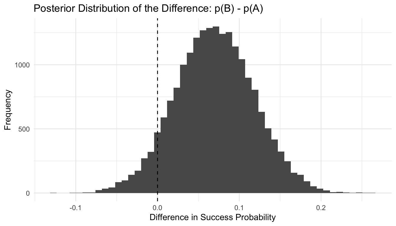
  • what is the probability model A is better than model B?
  • how uncertain are we about a slope, risk difference, or calibration parameter?

This is often more aligned with how scientists and decision-makers actually think.

They usually care less about a hypothetical repeated-sampling procedure and more about what the current data imply now.


A Medical Diagnosis Framing Makes the Logic Intuitive

A classic way to understand Bayesian thinking is through diagnosis.

Suppose a disease is rare. Even a good test can produce many false positives if the prior prevalence is low.

That means:

  • the test result alone is not enough,
  • and the prior probability of disease matters.

This is one of the places where Bayesian thinking is especially natural.

A positive test updates belief. It does not create belief from nothing.

That is also why Bayesian reasoning is so important in clinical decision-making and AI systems that operate in low-prevalence, high-uncertainty environments.


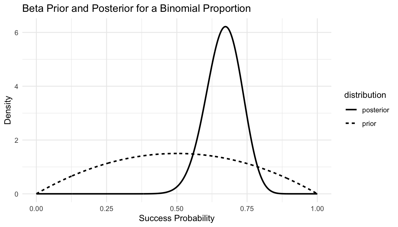
A Simple Beta-Binomial Example Shows Analytic Updating

One of the nicest Bayesian teaching examples is the Beta-Binomial model.

Suppose (y) successes are observed out of (n) trials, and the success probability is (p).

The likelihood is Binomial:

\[ y \mid p \sim \text{Binomial}(n, p) \]

Choose a Beta prior:

\[ p \sim \text{Beta}(\alpha, \beta) \]

Then the posterior is also Beta:

\[ p \mid y \sim \text{Beta}(\alpha + y, \beta + n - y) \]

This is called conjugacy.

The prior and posterior belong to the same family, which makes updating analytically simple.

library(dplyr)
library(tibble)
library(ggplot2)

n <- 50
y <- 34

alpha_prior <- 2
beta_prior  <- 2

alpha_post <- alpha_prior + y
beta_post  <- beta_prior + (n - y)

tibble::tibble(
  quantity = c("prior alpha", "prior beta", "posterior alpha", "posterior beta"),
  value = c(alpha_prior, beta_prior, alpha_post, beta_post)
)
# A tibble: 4 × 2
  quantity        value
  <chr>           <dbl>
1 prior alpha         2
2 prior beta          2
3 posterior alpha    36
4 posterior beta     18

Now visualize the prior and posterior.

p_grid <- seq(0, 1, length.out = 1000)

beta_df <- tibble::tibble(
  p = p_grid,
  prior = dbeta(p_grid, alpha_prior, beta_prior),
  posterior = dbeta(p_grid, alpha_post, beta_post)
) |>
  tidyr::pivot_longer(
    cols = c(prior, posterior),
    names_to = "distribution",
    values_to = "density"
  )

ggplot2::ggplot(beta_df, ggplot2::aes(x = p, y = density, linetype = distribution)) +
  ggplot2::geom_line(linewidth = 0.9) +
  ggplot2::labs(
    title = "Beta Prior and Posterior for a Binomial Proportion",
    x = "Success Probability",
    y = "Density"
  ) +
  ggplot2::theme_minimal()

This plot shows Bayesian learning clearly: the posterior reflects the prior updated by the observed data.


Conjugacy Makes Bayesian Updating Transparent

Conjugate priors are mathematically convenient because they keep posterior updating simple.

Common examples include:

  • Beta prior + Binomial likelihood
  • Gamma prior + Poisson likelihood
  • Normal prior + Normal likelihood

These examples are pedagogically useful because they show the logic of Bayesian updating without requiring advanced computation.

They also reveal something deeper:

Bayesian inference is often just structured accumulation of prior information and sample information.

Even when conjugacy does not hold exactly, the same logic remains. The only difference is that the posterior may need numerical approximation.


Priors Influence More When Data Are Sparse

One of the most important practical lessons in Bayesian inference is that priors matter most when data are limited.

With large datasets, the likelihood often dominates.

With small datasets, the prior can meaningfully shape the posterior.

That is not necessarily a weakness. In many small-sample settings, incorporating reasonable external knowledge is a strength.

This is especially relevant in:

  • pilot studies,
  • rare disease work,
  • subgroup analyses,
  • military or operational contexts with sparse events,
  • and ML settings where data are limited or imbalanced.

The real question is whether the prior is justified and transparent.


A Frequentist Contrast Helps Clarify the Difference

Suppose we observe 34 successes in 50 trials.

A frequentist might summarize this with:

  • a sample proportion,
  • a confidence interval,
  • and perhaps a hypothesis test.

A Bayesian would instead produce a posterior distribution for (p).

That allows direct statements such as:

  • the posterior mean of (p)
  • a 95% credible interval for (p)
  • the posterior probability that (p > 0.6)

Let us compute those.

posterior_mean <- alpha_post / (alpha_post + beta_post)
credible_interval <- qbeta(c(0.025, 0.975), alpha_post, beta_post)
prob_gt_060 <- 1 - pbeta(0.60, alpha_post, beta_post)

tibble::tibble(
  quantity = c("Posterior mean", "2.5% credible bound", "97.5% credible bound", "P(p > 0.60 | data)"),
  value = c(posterior_mean, credible_interval[1], credible_interval[2], prob_gt_060)
)
# A tibble: 4 × 2
  quantity             value
  <chr>                <dbl>
1 Posterior mean       0.667
2 2.5% credible bound  0.537
3 97.5% credible bound 0.785
4 P(p > 0.60 | data)   0.850

This is often a more natural inferential language than p-values alone.


Credible Intervals and Confidence Intervals Are Not the Same

A credible interval and a confidence interval can look numerically similar, but they mean different things (Morey et al. 2016; Kruschke 2015).

A 95% credible interval means:

given the model, prior, and observed data, there is 95% posterior probability that the parameter lies in this interval.

A 95% confidence interval means:

across repeated hypothetical samples, 95% of intervals constructed this way would contain the true parameter.

Those are different inferential statements.

Bayesian intervals are often easier to interpret because they align with how people naturally talk about uncertainty.

But they remain conditional on the model and prior.


A/B Testing Is a Natural Bayesian Use Case

Bayesian inference is especially appealing for A/B testing.

Instead of asking only whether the null hypothesis of equal performance can be rejected, Bayesian A/B testing can ask:

  • what is the posterior probability that B is better than A?
  • what is the posterior distribution of the difference?
  • how large is the likely advantage?
  • is the improvement operationally meaningful?

Let us simulate a simple example.

n_A <- 200
y_A <- 118

n_B <- 200
y_B <- 132

alpha_A_post <- 1 + y_A
beta_A_post  <- 1 + n_A - y_A

alpha_B_post <- 1 + y_B
beta_B_post  <- 1 + n_B - y_B

Draw from both posteriors and compare them.

n_draws <- 20000

draws_df <- tibble::tibble(
  p_A = rbeta(n_draws, alpha_A_post, beta_A_post),
  p_B = rbeta(n_draws, alpha_B_post, beta_B_post)
) |>
  dplyr::mutate(
    diff = p_B - p_A
  )

draws_df |>
  dplyr::summarise(
    prob_B_better = mean(diff > 0),
    mean_diff = mean(diff),
    ci_lower = quantile(diff, 0.025),
    ci_upper = quantile(diff, 0.975)
  )
# A tibble: 1 × 4
  prob_B_better mean_diff ci_lower ci_upper
          <dbl>     <dbl>    <dbl>    <dbl>
1         0.928    0.0697  -0.0253    0.164

And plot the posterior difference.

ggplot2::ggplot(draws_df, ggplot2::aes(x = diff)) +
  ggplot2::geom_histogram(bins = 50) +
  ggplot2::geom_vline(xintercept = 0, linetype = 2) +
  ggplot2::labs(
    title = "Posterior Distribution of the Difference: p(B) - p(A)",
    x = "Difference in Success Probability",
    y = "Frequency"
  ) +
  ggplot2::theme_minimal()

This is often more decision-relevant than a binary significance test.


Bayesian Inference Is Valuable in Small-Data Problems

One of the strongest use cases for Bayesian inference is limited data.

When sample sizes are small, purely data-driven estimates can be unstable.

Bayesian methods can help by:

  • regularizing extreme estimates,
  • incorporating prior knowledge,
  • producing full posterior uncertainty,
  • and avoiding overconfident point summaries.

This is particularly useful in biostats/ML hybrid settings where:

  • data are scarce,
  • prior knowledge is meaningful,
  • and decisions still need to be made.

That is one reason Bayesian methods often feel especially compelling in rare-event or subgroup problems.


MCMC Matters When Analytic Posteriors Are Not Available

Conjugate models are elegant, but many real models do not yield closed-form posteriors.

That is where Markov chain Monte Carlo (MCMC) comes in.

MCMC methods approximate posterior distributions by drawing samples from them computationally (Gelman et al. 2013; McElreath 2020).

This allows Bayesian inference for:

  • hierarchical models,
  • logistic regression with richer priors,
  • missing data models,
  • latent-variable models,
  • and many complex biostatistical and ML workflows.

For this post, the goal is not to fully teach MCMC, but to place it correctly:

MCMC is a computational strategy for approximating the posterior when algebra alone is not enough.


An Optional Simple MCMC-Style Example with rstanarm or brms

If you want to extend this post into a more applied Bayesian modeling workflow, you could fit a Bayesian regression model using rstanarm or brms.

Below is an optional code block you could enable if those packages are installed.

required_pkgs <- c("rstanarm")
missing_pkgs <- required_pkgs[
  !vapply(required_pkgs, requireNamespace, logical(1), quietly = TRUE)
$$

if (length(missing_pkgs) > 0) {
  stop("Missing packages: ", paste(missing_pkgs, collapse = ", "))
}

library(rstanarm)

reg_df <- tibble::tibble(
  x = rnorm(120, 50, 10),
  y = 5 + 0.8 * x + rnorm(120, 0, 6)
)

fit_bayes <- rstanarm::stan_glm(
  y ~ x,
  data = reg_df,
  family = gaussian(),
  refresh = 0
)

print(fit_bayes)
posterior_interval(fit_bayes)

This is a natural bridge from conjugate examples into full posterior computation.


Bayesian Thinking Also Matters in Modern AI/ML

Bayesian ideas extend far beyond classical data analysis.

They power or influence:

  • Bayesian optimization,
  • probabilistic deep learning,
  • variational inference,
  • uncertainty-aware prediction,
  • Gaussian processes,
  • and regularized small-data modeling.

Even when a method is not fully Bayesian, Bayesian thinking often shapes how uncertainty and prior structure are handled.

This matters because many AI systems still struggle with overconfidence.

Bayesian approaches are one route toward making predictive systems more honest about uncertainty.


Bayesian Inference Is Powerful, but Not Automatic

Bayesian methods are powerful, but they still require judgment.

Important considerations include:

  • prior choice,
  • model specification,
  • likelihood adequacy,
  • posterior sensitivity,
  • and computational diagnostics.

A Bayesian model can still be misleading if:

  • the prior is poorly chosen,
  • the likelihood is unrealistic,
  • or the computation has not converged properly.

So Bayesian inference should not be treated as a magic upgrade. It is a principled framework, but still one that depends on careful modeling.


A Practical Checklist for Applied Work

Before using or reporting a Bayesian analysis, ask:

  • What prior did I choose, and why?
  • Is the prior weakly informative, informative, or diffuse?
  • What is the likelihood model?
  • Is the posterior available analytically, or do I need MCMC?
  • How sensitive are the conclusions to the prior?
  • Would a frequentist summary tell a materially different story?
  • Is the Bayesian output more aligned with the real decision I need to make?

These questions often improve both transparency and interpretation.

NoteWhere This Shows Up in AI/ML

Bayesian neural networks — used in systems like the UK’s ACHD cardiac risk tool and in research trauma triage models — replace point-weight estimates with posterior distributions over weights, enabling the model to output a posterior predictive distribution for each patient rather than a single probability score; this means the model can communicate “I’m confident this patient is high-risk” versus “this patient’s risk is genuinely uncertain and you should not rely on this score alone.” When a trauma outcome model is deployed to a new operational environment (say, moving from CONUS hospital data to deployed DoDTR cases) without updating the prior, the posterior predictive distribution will be miscalibrated in proportion to how far the new population sits from the training population — a failure that Bayesian framing makes explicit and that purely frequentist models hide entirely.


Closing: Bayesian Inference Makes Uncertainty Explicit

Bayesian inference remains compelling because it treats learning as updating.

It gives a coherent structure for combining prior knowledge with observed data. It yields full posterior distributions rather than only point estimates. And it often speaks more directly to the real questions analysts and decision-makers want answered.

That is true in:

  • medical diagnosis,
  • A/B testing,
  • small-sample biostatistics,
  • and modern AI systems that need better uncertainty handling.

Bayesian inference matters because it turns uncertainty from an inconvenience into a first-class part of the model.


Tip📚 Go Deeper: Bayesian Workflow Toolkit

This post is part of the Bayesian Workflow Toolkit — a companion reference with prior justification templates, posterior predictive check code, credible interval reporting, and audit-ready Bayesian workflow scaffolds.

→ Open the Bayesian Workflow Toolkit


Series Callout

Note

This post is part of a broader Applied Statistics for AI and Clinical Decision-Making Series:

  • Probability fundamentals for machine learning
  • Random variables and expectation
  • Common probability distributions
  • Central Limit Theorem
  • Law of Large Numbers
  • Sampling methods for Biostats and ML
  • Hypothesis testing in the age of AI
  • Confidence intervals
  • Maximum likelihood estimation
  • Bayesian inference
  • Linear regression
  • Logistic regression
  • Generalized linear models
  • Analysis of variance
  • Principal component analysis
  • Cluster analysis
  • Time series analysis
  • Survival analysis
  • Non-parametric methods
  • Bias-variance tradeoff
  • Regularization
  • Cross-validation
  • Information theory
  • Optimization techniques
  • Linear algebra basics
  • Calculus for ML
  • Monte Carlo methods
  • Dimensionality curse and reduction techniques
  • Model evaluation metrics
  • Ensemble methods

References

Bayes, Thomas, and Richard Price. 1763. “An Essay Towards Solving a Problem in the Doctrine of Chances.” Philosophical Transactions of the Royal Society of London 53: 370–418. https://doi.org/10.1098/rstl.1763.0053.
Gelman, Andrew, John B. Carlin, Hal S. Stern, David B. Dunson, Aki Vehtari, and Donald B. Rubin. 2013. Bayesian Data Analysis. 3rd ed. Chapman; Hall/CRC.
Kruschke, John K. 2015. Doing Bayesian Data Analysis: A Tutorial with R, JAGS, and Stan. 2nd ed. Academic Press.
McElreath, Richard. 2020. Statistical Rethinking: A Bayesian Course with Examples in R and Stan. 2nd ed. CRC Press. https://doi.org/10.1201/9780429029608.
Morey, Richard D., Rink Hoekstra, Jeffrey N. Rouder, Michael D. Lee, and Eric-Jan Wagenmakers. 2016. “The Fallacy of Placing Confidence in Confidence Intervals.” Psychonomic Bulletin & Review 23 (1): 103–23. https://doi.org/10.3758/s13423-015-0947-8.