Linear Regression Still Matters: The Workhorse Model Behind AI and Biostats
Applied Statistics
Linear Regression
An applied introduction to linear regression, ordinary least squares, assumptions, diagnostics, and prediction for AI and clinical data analysis.
Published
January 15, 2024
Modified
June 9, 2026
Executive Summary
Linear regression is one of the most familiar tools in statistics, but it is also one of the most important conceptual bridges into machine learning.
At first glance, it can look almost too simple:
fit a line,
estimate coefficients,
report p-values,
quote an (\(R^2\)),
move on.
But that view misses why linear regression matters.
Linear regression teaches some of the most important ideas in quantitative modeling:
how predictors relate to outcomes,
how model parameters are estimated,
how assumptions shape interpretation,
how uncertainty enters fitted models,
and how prediction differs from explanation.
It also sits underneath a surprising amount of modern AI/ML thinking.
Linear regression is closely connected to:
least-squares optimization,
generalized linear models,
regularization,
feature engineering,
and even the logic of neural networks.
This post walks through linear regression from an applied perspective, with a biostatistical flavor and an ML framing.
We will cover:
fitting models with ordinary least squares,
interpreting coefficients,
checking assumptions,
understanding (\(R^2\)),
and diagnosing multicollinearity.
Linear regression is not obsolete because it is simple. It is foundational because it teaches the structure of modeling clearly.
Linear Regression Is About Modeling Average Relationships
Linear regression models the expected value of an outcome as a function of one or more predictors.
In its simplest form:
\[
Y_i = \beta_0 + \beta_1 X_i + \varepsilon_i
\]
where:
\(Y_i\) is the outcome
\(X_i\) is the predictor
\(\beta_0\) is the intercept
\(\beta_1\) is the slope
and (_i) captures unexplained variability.
The key idea is not that every observation lies exactly on a line.
The key idea is that the average outcome changes systematically with the predictor.
That makes linear regression a model of expected structure, not exact determinism.
Why Linear Regression Still Matters in AI/ML
Linear regression remains important because it teaches the core logic of supervised learning in a transparent way.
It introduces:
parametric prediction,
optimization of an objective function,
trainable coefficients,
fitted values and residuals,
and the tradeoff between signal and noise.
In many ways, it is the cleanest entry point into ideas that later reappear in:
logistic regression,
penalized models like ridge and lasso,
generalized linear models,
boosted linear learners,
and neural network layers.
If someone understands linear regression deeply, they usually understand much more about modeling than they first realize.
A Simple Biostats-Style Example
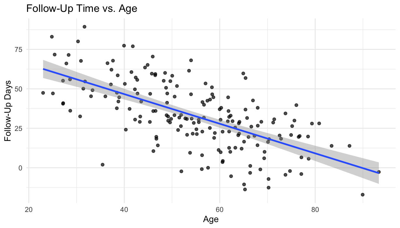
To keep the workflow concrete, we will simulate a simple biostats-style dataset with a continuous outcome that could be interpreted as a survival-related or follow-up-type measure.
Here, the outcome will be a continuous proxy such as days to recovery or follow-up time, modeled as a function of age and severity score.
library(dplyr)library(tibble)library(ggplot2)n <-180reg_df <- tibble::tibble(age =rnorm(n, mean =55, sd =14),severity =rnorm(n, mean =10, sd =3)) |> dplyr::mutate(followup_days =120-0.9* age -3.5* severity +rnorm(n, mean =0, sd =12) )reg_df |> dplyr::summarise(n = dplyr::n(),mean_age =mean(age),mean_severity =mean(severity),mean_followup =mean(followup_days) )
# A tibble: 1 × 4
      n mean_age mean_severity mean_followup
  <int>    <dbl>         <dbl>         <dbl>
1   180     54.6          10.2          32.9
This is only a teaching example, but it provides a useful stand-in for a clinical outcome that varies with patient characteristics.
Fitting a Linear Regression Model with OLS
Ordinary least squares, or OLS, estimates regression coefficients by minimizing the sum of squared residuals.
A residual is:
\[
e_i = y_i - \hat{y}_i
\]
OLS chooses the coefficients that make the total squared residual error as small as possible.
We can fit the model in R with lm().
fit_lm <-lm(followup_days ~ age + severity, data = reg_df)summary(fit_lm)
Call:
lm(formula = followup_days ~ age + severity, data = reg_df)

Residuals:
     Min       1Q   Median       3Q      Max
-30.2906  -6.6378   0.8329   8.2609  29.6800

Coefficients:
            Estimate Std. Error t value Pr(>|t|)
(Intercept) 122.9424     4.5223   27.19   <2e-16 ***
age          -0.9174     0.0600  -15.29   <2e-16 ***
severity     -3.8952     0.3007  -12.95   <2e-16 ***
---
Signif. codes:  0 '***' 0.001 '**' 0.01 '*' 0.05 '.' 0.1 ' ' 1

Residual standard error: 11.77 on 177 degrees of freedom
Multiple R-squared:  0.6997,    Adjusted R-squared:  0.6964
F-statistic: 206.3 on 2 and 177 DF,  p-value: < 2.2e-16
and approximate normality of residuals for some inferential procedures.
These assumptions do not all matter in exactly the same way.
Some matter more for unbiased estimation. Some matter more for standard errors and inference. Some matter more for prediction quality.
But if they are badly violated, the model can become misleading.
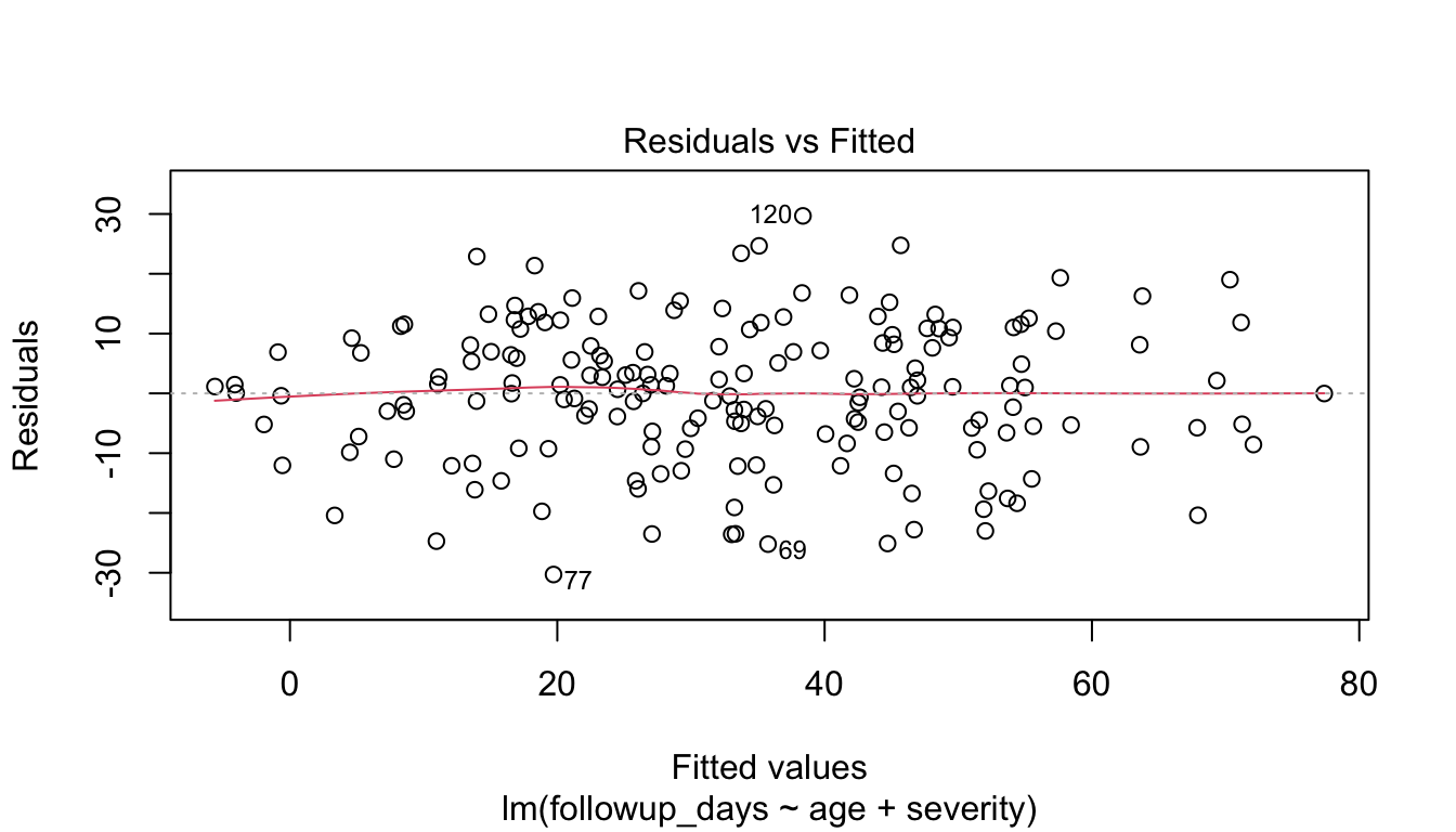
Checking Linearity with Residual Plots
A common question is whether the relationship between predictors and the outcome is adequately linear.
One simple diagnostic is the residual-versus-fitted plot.
plot(fit_lm, which =1)
In a well-behaved linear model, residuals should look roughly centered around zero without strong systematic curvature.
If there is strong patterning, the model may be missing nonlinear structure.
That does not automatically invalidate the analysis, but it suggests the linear form may be incomplete.
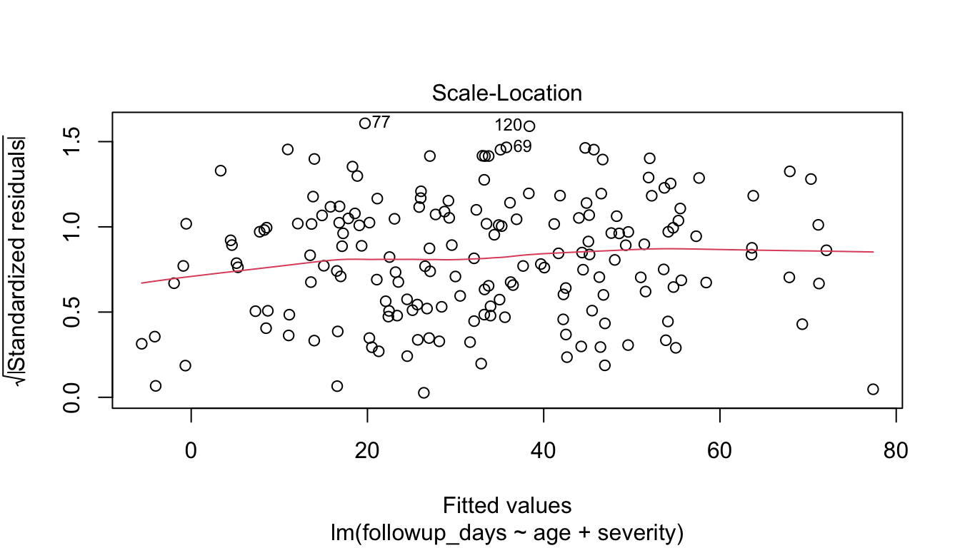
Checking Homoscedasticity Means Checking Variance Stability
Homoscedasticity means the residual variance is roughly constant across fitted values.
When variance changes systematically with the level of the fitted outcome, we have heteroscedasticity.
This matters because heteroscedasticity can distort standard errors and reduce the reliability of classical inference.
Again, the residual-versus-fitted plot is helpful.
We can also look at a scale-location plot.
plot(fit_lm, which =3)
A strong funnel shape would suggest nonconstant variance.
In applied work, this may motivate:
transformations,
robust standard errors,
alternative modeling strategies,
or more flexible mean-variance structures.
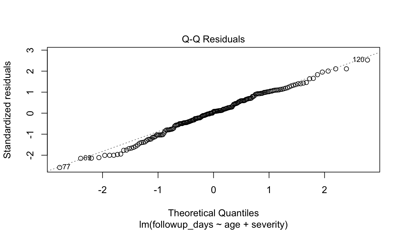
Normality of Residuals Is Often Overemphasized, but Still Useful to Check
Residual normality is one of the most talked-about assumptions, though in many settings it is not the most critical one.
Still, it is often useful to inspect.
plot(fit_lm, which =2)
If the residuals are roughly aligned with the reference line, the normal approximation is often adequate for standard inference.
Small deviations are not unusual. What matters is whether the departures are large enough to affect interpretation materially.
In modern applied work, analysts should avoid treating perfect normality as a sacred requirement, but they should still check whether the model appears grossly inconsistent with the data.
Interpreting (\(R^2\)) Requires Restraint
The coefficient of determination, (\(R^2\)), is often treated as a summary of model quality.
It measures the proportion of variance in the outcome explained by the model, at least in a classical decomposition sense.
That can be useful. But (\(R^2\)) is not a universal score of scientific value.
A model can have:
a modest (\(R^2\)) and still contain highly meaningful predictors,
or a high (\(R^2\)) and still be scientifically shallow or operationally unhelpful.
We can extract the model (\(R^2\)) directly.
summary(fit_lm)$r.squared
[1] 0.699748
summary(fit_lm)$adj.r.squared
[1] 0.6963553
Adjusted (\(R^2\)) is often preferable when comparing models with different numbers of predictors.
But even then, it should not replace substantive interpretation.
Predicted Values and Residuals Teach How the Model Behaves
A fitted regression model produces predicted values:
\[
\hat{y}_i
\]
and residuals:
\[
e_i = y_i - \hat{y}_i
\]
These two quantities are central for understanding model behavior.
VIFs do not produce a magical cutoff that solves the problem, but they are helpful for identifying when predictor overlap may be inflating uncertainty.
Linear Regression Is Also a Baseline Model in ML
In machine learning, linear regression is often used as a baseline.
That matters because a baseline model helps answer an important question:
does a more complex model actually improve meaningfully on a simple, interpretable benchmark?
This is one reason linear regression remains valuable even when more flexible methods are available.
It provides:
a transparent benchmark,
interpretable coefficients,
fast fitting,
and a useful reference point for more complex learners.
If a sophisticated model cannot clearly outperform a thoughtful linear baseline, that is often diagnostically important.
Regression Assumptions Are Not Just Technicalities
One of the dangers in teaching regression is making the assumptions look like an afterthought.
They are not.
Assumptions shape:
what the coefficients mean,
whether standard errors are reliable,
whether fitted values extrapolate sensibly,
and how much trust we can place in the resulting inference.
This is especially important in biostatistics, where a regression table can appear authoritative even when the model fit is poor or the assumptions are badly strained.
Model diagnostics are therefore part of the analysis, not decoration after the fact.
A Small Prediction Example
To keep the ML connection concrete, we can use the fitted model to generate a predicted follow-up time for a hypothetical patient.
the confidence interval is for the expected mean outcome at those predictor values
the prediction interval is for an individual future observation
The prediction interval is wider because individual patients vary around the mean.
That distinction matters greatly in both clinical prediction and AI deployment.
Linear Regression Is the Gateway to More Advanced Models
Many “next-step” models are easiest to understand after mastering linear regression.
These include:
logistic regression,
Poisson regression,
Cox models,
ridge and lasso regression,
mixed models,
Bayesian regression,
and neural network layers with learned weights.
What changes across these models is often:
the outcome distribution,
the link function,
the penalty structure,
or the dependence structure.
But the core modeling idea remains recognizable.
That is why linear regression is such an important gateway.
A Practical Checklist for Applied Work
Before reporting a linear regression model, ask:
Is the mean structure plausibly linear?
Are the coefficients being interpreted conditionally and correctly?
Are residual plots broadly consistent with the assumptions?
Is variance roughly stable?
Are the predictors strongly collinear?
Is (\(R^2\)) being interpreted with restraint?
Is the model being used for explanation, prediction, or both?
Would a simpler or more flexible model be more appropriate?
These questions often matter more than the regression table itself.
NoteWhere This Shows Up in AI/ML
Every dense layer in a neural network is a linear regression: a weighted sum of inputs passed through an activation function, with weights learned by minimizing a loss. When OLS assumptions break in EHR-based prediction — heteroscedasticity from differential documentation intensity across facilities, or correlated errors from repeated patient encounters — standard errors become unreliable and model confidence intervals mislead downstream decision-makers. In military health, regression to the mean is a recurring trap: patients selected for high severity at injury often look like they “improved” at follow-up even without intervention, inflating apparent treatment effects in DoDTR outcome models. Ignoring this artifact leads to deployment of protocols that appear effective in training data but produce no real benefit in theater.
Closing: Linear Regression Still Teaches the Core Logic of Modeling
Linear regression endures because it teaches so much with relatively little machinery.
It shows how models connect predictors to outcomes. It shows how parameters are estimated through optimization. It forces attention to assumptions. It reveals the distinction between explained structure and residual variability.
And it prepares analysts for more advanced methods in both statistics and machine learning.
Linear regression remains one of the best places to learn modeling well, because it makes the architecture of prediction and inference visible.
This post is part of the Prediction Modeling Toolkit — a companion reference with regression assumption check templates, residual diagnostic code, and coefficient reporting scaffolds.
Harrell, Jr., Frank E. 2015. Regression Modeling Strategies. 2nd ed. Springer.
Hastie, Trevor, Robert Tibshirani, and Jerome Friedman. 2009. The Elements of Statistical Learning: Data Mining, Inference, and Prediction. 2nd ed. Springer.
James, Gareth, Daniela Witten, Trevor Hastie, and Robert Tibshirani. 2021. An Introduction to Statistical Learning: With Applications in R. 2nd ed. Springer.
Murphy, Kevin P. 2012. Machine Learning: A Probabilistic Perspective. MIT Press.
Wasserman, Larry. 2004. All of Statistics: A Concise Course in Statistical Inference. Springer.