Logistic Regression: Predicting Yes/No in AI and Beyond

An applied introduction to logistic regression, odds ratios, ROC/AUC, classification thresholds, and regularization for AI and clinical prediction.

Executive Summary

Many important problems in statistics and machine learning are not about predicting a continuous quantity.

They are about predicting a yes/no outcome.

Examples include:

• disease vs. no disease,
• mortality vs. survival,
• fraud vs. no fraud,
• click vs. no click,
• response vs. nonresponse,
• success vs. failure.

This is where logistic regression becomes one of the most useful and enduring models in applied analytics (McCullagh and Nelder 1989; Hosmer et al. 2013; James et al. 2021).

Logistic regression is often introduced as a “simple classifier,” but that undersells its importance.

It teaches:

• how to model probabilities,
• how link functions work,
• how classification differs from regression,
• how decision thresholds affect performance,
• and how regularization stabilizes models in higher-dimensional settings.

It also remains a core bridge between classical biostatistics and modern AI/ML.

This post introduces:

• binary outcome modeling,
• the logit link,
• coefficient interpretation,
• confusion matrices,
• ROC/AUC evaluation,
• and L1/L2 regularization.

Logistic regression matters because it turns binary decision problems into interpretable probability models.

---

Logistic Regression Models Probability, Not Just Labels

A binary outcome can be coded as:

• 1 = event occurred
• 0 = event did not occur

But the real modeling target is usually not only the label. It is the probability of the event.

That is a crucial distinction.

A classifier that only outputs yes/no decisions hides uncertainty. A logistic regression model instead estimates:

\[ P(Y = 1 \mid X) \]

This is often much more useful.

It allows us to ask:

• how likely is the event?
• how does risk change with predictors?
• what threshold should trigger action?
• how uncertain or calibrated are the predictions?

That is why logistic regression remains central in clinical prediction, risk modeling, and ML classification (Hosmer et al. 2013; Steyerberg 2019).

---

Why Ordinary Linear Regression Is Not Enough for Binary Outcomes

It may be tempting to model a binary outcome using ordinary linear regression.

But that creates several problems.

A linear model can produce fitted values below 0 or above 1, which are invalid as probabilities.

It also assumes a constant marginal change in the outcome, which does not reflect how probabilities behave near the boundaries.

Binary outcomes need a model that:

• keeps predicted probabilities between 0 and 1,
• allows nonlinear probability behavior,
• and links predictors to the event probability in a coherent way.

That is exactly what logistic regression does.

---

The Logit Link Connects Predictors to Event Probability

Logistic regression models the probability of an event through the logit link (McCullagh and Nelder 1989; Hosmer et al. 2013).

Let:

\[ \pi_i = P(Y_i = 1 \mid X_i) \]

The model is:

\[ \log\left(\frac{\pi_i}{1 - \pi_i}\right) = \beta_0 + \beta_1 X_{i1} + \cdots + \beta_p X_{ip} \]

The quantity

\[ \frac{\pi_i}{1 - \pi_i} \]

is the odds of the event.

Taking the log of the odds gives the log-odds, or logit.

This transformation maps probabilities from \((0, 1)\) to the full real line, which makes linear modeling possible on the transformed scale.

That is the key idea.

Logistic regression is linear in the log-odds, not in the raw probability.

---

A Biostats-Style Example Makes the Model Concrete

We will simulate a simple biostatistical example in which the outcome is a binary event such as a complication, response, or deterioration indicator.

We will model that outcome using age and a severity score.

library(dplyr)
library(tibble)
library(ggplot2)

n <- 300

logit_df <- tibble::tibble(
  age = rnorm(n, mean = 55, sd = 12),
  severity = rnorm(n, mean = 10, sd = 3)
) |>
  dplyr::mutate(
    linpred = -6 + 0.05 * age + 0.35 * severity,
    prob = 1 / (1 + exp(-linpred)),
    event = rbinom(n, size = 1, prob = prob)
  )

logit_df |>
  dplyr::summarise(
    n = dplyr::n(),
    event_rate = mean(event),
    mean_age = mean(age),
    mean_severity = mean(severity)
  )

# A tibble: 1 × 4
      n event_rate mean_age mean_severity
  <int>      <dbl>    <dbl>         <dbl>
1   300      0.543     54.6          9.84

This gives us a realistic binary-outcome setting for illustration.

---

Fitting a Logistic Regression Model

In R, logistic regression is fit with glm() using the binomial family (McCullagh and Nelder 1989; Hosmer et al. 2013).

fit_logit <- glm(
  event ~ age + severity,
  data = logit_df,
  family = binomial()
)

summary(fit_logit)

Call:
glm(formula = event ~ age + severity, family = binomial(), data = logit_df)

Coefficients:
            Estimate Std. Error z value Pr(>|z|)    
(Intercept) -6.62678    0.97782  -6.777 1.23e-11 ***
age          0.05255    0.01187   4.427 9.56e-06 ***
severity     0.40365    0.05745   7.026 2.12e-12 ***
---
Signif. codes:  0 '***' 0.001 '**' 0.01 '*' 0.05 '.' 0.1 ' ' 1

(Dispersion parameter for binomial family taken to be 1)

    Null deviance: 413.63  on 299  degrees of freedom
Residual deviance: 329.28  on 297  degrees of freedom
AIC: 335.28

Number of Fisher Scoring iterations: 4

This output provides:

• regression coefficients on the log-odds scale,
• standard errors,
• z-statistics,
• and p-values.

But interpreting coefficients directly on the log-odds scale can feel abstract.

That is why odds ratios are often used.

---

Coefficients Are Interpreted Through Odds Ratios

Each logistic regression coefficient represents the expected change in the log-odds of the outcome per one-unit increase in the predictor, holding other predictors constant.

Exponentiating a coefficient gives an odds ratio (Hosmer et al. 2013).

or_tbl <- tibble::tibble(
  term = names(coef(fit_logit)),
  estimate = coef(fit_logit),
  odds_ratio = exp(coef(fit_logit))
)

or_tbl

# A tibble: 3 × 3
  term        estimate odds_ratio
  <chr>          <dbl>      <dbl>
1 (Intercept)  -6.63      0.00132
2 age           0.0526    1.05   
3 severity      0.404     1.50   

Interpretation example:

• if the odds ratio for severity is greater than 1, higher severity is associated with higher odds of the event
• if the odds ratio for age is close to 1, age may have a smaller per-unit effect

This is a conditional interpretation, just as in linear regression.

Each coefficient is interpreted holding the other variables constant.

---

Predicted Probabilities Are Often More Intuitive Than Odds Ratios

Odds ratios are useful, but many readers understand predicted probabilities more easily.

We can generate predicted probabilities for each observation.

logit_df <- logit_df |>
  dplyr::mutate(
    pred_prob = predict(fit_logit, type = "response")
  )

logit_df |>
  dplyr::select(age, severity, event, pred_prob) |>
  dplyr::slice_head(n = 10)

# A tibble: 10 × 4
     age severity event pred_prob
   <dbl>    <dbl> <int>     <dbl>
 1  63.7     9.05     0     0.592
 2  46.3     9.03     0     0.367
 3  56.2    11.2      1     0.701
 4  41.0    13.8      1     0.750
 5  31.7    10.2      0     0.304
 6  55.2     6.95     0     0.285
 7  67.3    11.0      1     0.794
 8  50.4    14.9      1     0.884
 9  38.8     7.53     0     0.175
10  57.1     8.30     1     0.431

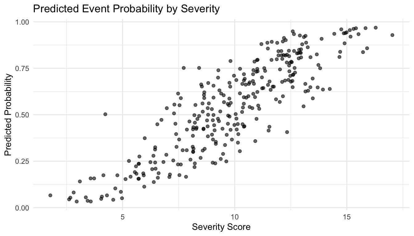
We can also visualize how predicted probability changes with severity while holding age roughly constant through a simple plot.

ggplot2::ggplot(logit_df, ggplot2::aes(x = severity, y = pred_prob)) +
  ggplot2::geom_point(alpha = 0.6) +
  ggplot2::labs(
    title = "Predicted Event Probability by Severity",
    x = "Severity Score",
    y = "Predicted Probability"
  ) +
  ggplot2::theme_minimal()

This helps connect model coefficients to clinical or operational risk.

---

Logistic Regression Is Trained by Maximum Likelihood

Logistic regression is not fit by ordinary least squares.

It is estimated by maximum likelihood.

That is important because it links logistic regression directly to the broader ML idea of optimizing an objective function (Murphy 2012; Hastie et al. 2009).

The model parameters are chosen to maximize the likelihood of the observed binary outcomes under the Bernoulli model.

Equivalently, many ML workflows describe this as minimizing log loss or cross-entropy loss.

That is one reason logistic regression is such an important bridge between statistical modeling and machine learning.

---

Classification Requires a Threshold, Not Just a Probability Model

A logistic regression model outputs probabilities. To turn those into class labels, we need a threshold.

A common default is 0.50:

• predict 1 if predicted probability >= 0.50
• predict 0 otherwise

But that threshold is not always optimal.

In clinical or operational settings, the best threshold depends on:

• class imbalance,
• false positive cost,
• false negative cost,
• and decision context.

We can start with a 0.50 threshold to illustrate classification.

logit_df <- logit_df |>
  dplyr::mutate(
    pred_class = if_else(pred_prob >= 0.50, 1, 0)
  )

table(Predicted = logit_df$pred_class, Observed = logit_df$event)

         Observed
Predicted   0   1
        0  88  39
        1  49 124

That table is the basis of the confusion matrix.

---

The Confusion Matrix Summarizes Classification Performance

The confusion matrix is one of the simplest and most useful classification summaries (James et al. 2021).

It contains:

• true positives,
• true negatives,
• false positives,
• false negatives.

cm_tbl <- table(Predicted = logit_df$pred_class, Observed = logit_df$event)
cm_tbl

         Observed
Predicted   0   1
        0  88  39
        1  49 124

tp <- cm_tbl["1", "1"]
tn <- cm_tbl["0", "0"]
fp <- cm_tbl["1", "0"]
fn <- cm_tbl["0", "1"]

perf_tbl <- tibble::tibble(
  metric = c("Accuracy", "Sensitivity", "Specificity"),
  value = c(
    (tp + tn) / sum(cm_tbl),
    tp / (tp + fn),
    tn / (tn + fp)
  )
)

perf_tbl

# A tibble: 3 × 2
  metric      value
  <chr>       <dbl>
1 Accuracy    0.707
2 Sensitivity 0.761
3 Specificity 0.642

This is often more operationally meaningful than coefficients alone.

In ML, classification performance is not only about fitting the model, but also about how predictions behave after thresholding.

---

ROC Curves Show Performance Across All Thresholds

A confusion matrix depends on a single threshold. A ROC curve evaluates classification performance across many thresholds.

The ROC curve plots (Hosmer et al. 2013; Steyerberg 2019):

• sensitivity on the y-axis
• 1 - specificity on the x-axis

This gives a threshold-independent view of discrimination.

required_pkgs <- c("pROC")
missing_pkgs <- required_pkgs[
  !vapply(required_pkgs, requireNamespace, logical(1), quietly = TRUE)
$$

if (length(missing_pkgs) > 0) {
  stop("Missing packages: ", paste(missing_pkgs, collapse = ", "))
}

roc_obj <- pROC::roc(logit_df$event, logit_df$pred_prob)
plot(roc_obj)
pROC::auc(roc_obj)

The ROC framework is especially useful when the relative cost of false positives and false negatives is still being considered.

---

AUC Summarizes Discrimination, but Not Everything

The area under the ROC curve (AUC) is a common performance summary (Steyerberg 2019).

It represents the probability that a randomly chosen positive case receives a higher predicted score than a randomly chosen negative case.

That makes it a useful discrimination metric.

But AUC has limits.

A model can have:

• a decent AUC but poor calibration,
• a high AUC but poor threshold-specific utility,
• or a good AUC that masks subgroup performance issues.

So AUC is helpful, but it is not a complete description of model quality.

That is especially important in AI/ML, where a single metric can encourage false confidence.

---

Logistic Regression Assumes Linearity on the Logit Scale

One of the most important modeling assumptions is often overlooked:

logistic regression assumes that predictors relate linearly to the log-odds, not necessarily to the raw probability.

That means a predictor may appear to have a nonlinear effect on probability even when the model is correctly specified.

If the true relationship is more complex, simple logistic regression may be misspecified.

In applied work, this can motivate:

• transformations,
• interaction terms,
• splines,
• or more flexible classifiers.

So logistic regression is powerful, but it is not infinitely flexible.

---

Logistic Regression Can Be Extended with Interactions and Nonlinearity

A basic logistic model is often only the beginning.

Analysts frequently extend it by adding:

• interaction terms,
• polynomial terms,
• spline terms,
• or hierarchical structures.

For example, severity may matter differently at different ages.

That is an interaction question.

The simple model is still useful, but it should not be treated as the only possible specification.

This is one reason logistic regression remains such a good teaching tool: it shows clearly how model structure shapes inference and prediction.

---

L2 Regularization Shrinks Coefficients for Stability

When predictors are numerous or correlated, ordinary logistic regression can become unstable.

This is where regularization becomes valuable.

L2 regularization, often called ridge-style penalization, adds a penalty proportional to the squared coefficient magnitudes.

Conceptually, it says:

large coefficients should be discouraged unless the data strongly support them.

This can improve stability, reduce variance, and help with multicollinearity (Hastie et al. 2009; James et al. 2021).

In ML, regularization is one of the main ways to make models less fragile.

---

L1 Regularization Encourages Sparsity

L1 regularization, often called lasso-style penalization, adds a penalty proportional to the absolute coefficient magnitudes.

This tends to shrink some coefficients exactly to zero.

That makes L1 useful when:

• there are many predictors,
• some may be weak or irrelevant,
• and variable selection is desirable.

This is especially important in high-dimensional ML settings (Hastie et al. 2009; Murphy 2012).

L1 and L2 are both valuable, but they serve slightly different goals:

• L2 stabilizes
• L1 stabilizes and selects

---

A Penalized Logistic Regression Example

Below is an optional example using glmnet for penalized logistic regression.

required_pkgs <- c("glmnet")
missing_pkgs <- required_pkgs[
  !vapply(required_pkgs, requireNamespace, logical(1), quietly = TRUE)
$$

if (length(missing_pkgs) > 0) {
  stop("Missing packages: ", paste(missing_pkgs, collapse = ", "))
}

x_mat <- model.matrix(event ~ age + severity, data = logit_df)[, -1]
y_vec <- logit_df$event

fit_lasso <- glmnet::cv.glmnet(
  x = x_mat,
  y = y_vec,
  family = "binomial",
  alpha = 1
)

fit_ridge <- glmnet::cv.glmnet(
  x = x_mat,
  y = y_vec,
  family = "binomial",
  alpha = 0
)

coef(fit_lasso, s = "lambda.min")
coef(fit_ridge, s = "lambda.min")

This is a natural bridge from classical logistic regression into modern ML practice.

---

Logistic Regression Remains a Strong Baseline Classifier

In AI/ML, logistic regression is often used as a baseline model.

That is not because it is primitive. It is because it is:

• interpretable,
• fast,
• probabilistic,
• and surprisingly strong in many structured-data problems.

If a much more complex model cannot clearly outperform a logistic baseline, that is meaningful.

This is one reason logistic regression remains central in applied classification work, even in the era of deep learning.

---

Logistic Regression Also Generalizes Beyond Binary Outcomes

The importance of logistic regression extends further than yes/no classification.

It connects naturally to:

• multinomial logistic regression for multi-class outcomes,
• ordinal logistic models,
• softmax classifiers in NLP and deep learning,
• and output layers in neural network architectures.

So even when the specific model changes, the core idea remains familiar:

• model class probabilities,
• connect predictors through a link,
• optimize a probabilistic loss.

That is why logistic regression is such a durable conceptual anchor.

---

A Practical Checklist for Applied Work

Before reporting or deploying a logistic regression model, ask:

• Is the outcome truly binary and clearly defined?
• Are the coefficients being interpreted on the correct scale?
• Would predicted probabilities be more useful than odds ratios?
• Is the threshold appropriate for the decision context?
• Have I examined confusion-matrix behavior, not just coefficients?
• Have I assessed ROC/AUC with appropriate restraint?
• Is regularization needed because of predictor count or collinearity?
• Am I using logistic regression as a baseline, an explanatory model, or both?

These questions often matter more than whether the model “ran successfully.”

---

NoteWhere This Shows Up in AI/ML

The Epic Deterioration Index is a logistic regression model at its core: it outputs a probability that a patient will deteriorate within 24 hours, trained on EHR vitals, labs, and nursing flowsheet data. The threshold selection problem is where this gets clinically consequential — in military trauma triage, a threshold tuned to minimize false negatives in a Level I trauma center may flood a far-forward surgical team with low-acuity alerts, degrading trust and causing alert fatigue. AUC alone is insufficient here: a model with AUC of 0.82 can still be operationally useless if its calibration is poor or its sensitivity at the operationally relevant threshold is unacceptable. Models deployed in TCCC or en route care contexts must be validated against the specific threshold performance the operational scenario demands, not just ranked discrimination.

Closing: Logistic Regression Still Teaches the Core Logic of Classification

Logistic regression remains one of the best ways to learn binary classification properly.

It shows how to:

• model probabilities,
• connect predictors to risk,
• interpret coefficients conditionally,
• evaluate threshold-based decisions,
• and stabilize models through regularization.

It is useful in biostatistics because it is interpretable and principled. It is useful in machine learning because it is a core classifier and a gateway to broader predictive systems.

Logistic regression endures because it is simple enough to understand clearly, yet rich enough to teach the essential logic of classification in modern analytics.

---

Tip📚 Go Deeper: Prediction Modeling Toolkit

This post is part of the Prediction Modeling Toolkit — a companion reference with logistic regression templates, calibration plots, ROC curve code, and clinical prediction model reporting scaffolds.

→ Open the Prediction Modeling Toolkit

---

Series Callout

Note

This post is part of a broader Applied Statistics for AI and Clinical Decision-Making Series:

• Probability fundamentals for machine learning
• Random variables and expectation
• Common probability distributions
• Central Limit Theorem
• Law of Large Numbers
• Sampling methods for Biostats and ML
• Hypothesis testing in the age of AI
• Confidence intervals
• Maximum likelihood estimation
• Bayesian inference
• Linear regression
• Logistic regression
• Generalized linear models
• Analysis of variance
• Principal component analysis
• Cluster analysis
• Time series analysis
• Survival analysis
• Non-parametric methods
• Bias-variance tradeoff
• Regularization
• Cross-validation
• Information theory
• Optimization techniques
• Linear algebra basics
• Calculus for ML
• Monte Carlo methods
• Dimensionality curse and reduction techniques
• Model evaluation metrics
• Ensemble methods

Series: Applied Statistics for AI & Clinical Decision-Making

← Linear Regression Still Matters: The Workhorse Model Behind AI and Biostats  |  GLMs: Flexible Modeling for Real-World AI Data →

References

Hastie, Trevor, Robert Tibshirani, and Jerome Friedman. 2009. The Elements of Statistical Learning: Data Mining, Inference, and Prediction. 2nd ed. Springer.

Hosmer, David W., Stanley Lemeshow, and Rodney X. Sturdivant. 2013. Applied Logistic Regression. 3rd ed. Wiley.

James, Gareth, Daniela Witten, Trevor Hastie, and Robert Tibshirani. 2021. An Introduction to Statistical Learning: With Applications in R. 2nd ed. Springer.

McCullagh, Peter, and John A. Nelder. 1989. Generalized Linear Models. 2nd ed. Chapman; Hall.

Murphy, Kevin P. 2012. Machine Learning: A Probabilistic Perspective. MIT Press.

Steyerberg, Ewout W. 2019. Clinical Prediction Models: A Practical Approach to Development, Validation, and Updating. 2nd ed. Springer.