GLMs: Flexible Modeling for Real-World AI Data

Applied Statistics

Generalized Linear Models

An applied introduction to generalized linear models, link functions, binomial and Poisson regression, offsets, and overdispersion for AI and healthcare data.

Published

March 15, 2024

Modified

June 9, 2026

Executive Summary

Classical linear regression is powerful, but it assumes a continuous outcome with roughly normal errors and constant variance.

Many real-world data problems do not look like that at all.

Instead, we often encounter outcomes such as:

binary events,
counts,
rates,
proportions,
or strictly positive skewed measurements.

These outcomes do not fit comfortably into the assumptions of ordinary least squares.

This is where generalized linear models, or GLMs, become essential.

GLMs extend the logic of regression by allowing:

response distributions from the exponential family,
link functions that connect the mean response to predictors,
and variance structures that depend on the mean.

That makes GLMs one of the most important bridges between classical biostatistics and modern machine learning (Nelder and Wedderburn 1972; McCullagh and Nelder 1989; James et al. 2021).

This post introduces:

the basic structure of GLMs,
the role of the exponential family,
binomial and Poisson GLMs,
overdispersion,
and why GLMs remain foundational for applied AI/ML pipelines.

GLMs matter because real data are often not normal, and good modeling starts by matching the outcome structure to the model.

GLMs Extend Regression Beyond Normal Outcomes

Ordinary linear regression models a continuous outcome using a linear mean structure and normal-error assumptions.

That works well in some settings, but many outcomes do not behave that way.

Examples include:

whether a patient deteriorates,
how many infections occur,
how many clicks an ad receives,
how many admissions occur per week,
or how many complications are recorded per facility.

These outcomes are often:

bounded,
discrete,
skewed,
and mean-dependent in their variability.

GLMs generalize regression so that the response model better matches the actual data-generating structure (Nelder and Wedderburn 1972; McCullagh and Nelder 1989).

A GLM Has Three Core Components

A generalized linear model can be understood through three parts (Nelder and Wedderburn 1972; McCullagh and Nelder 1989).

Random Component

The response variable is assumed to follow a distribution from the exponential family, such as:

Normal
Binomial
Poisson
Gamma

Systematic Component

A linear predictor is formed:

\[ \eta_i = \beta_0 + \beta_1 X_{i1} + \cdots + \beta_p X_{ip} \]

Link Function

A link function connects the expected value of the response to the linear predictor:

\[ g(\mu_i) = \eta_i \]

where (_i = E(Y_i X_i)).

This structure is what makes GLMs so flexible.

The predictor can remain linear in the coefficients, while the outcome distribution and scale of the mean can change appropriately.

The Exponential Family Is the Mathematical Backbone

The phrase exponential family can sound abstract, but it is practically important because many useful data models belong to it.

Common examples include:

Normal for continuous outcomes
Binomial for binary outcomes or grouped proportions
Poisson for counts
Gamma for positive skewed outcomes

These models share a common mathematical structure that makes likelihood-based estimation and inference tractable.

In practice, this matters because GLMs preserve a coherent estimation framework while expanding beyond normal outcomes.

This is one reason GLMs are so central in statistics and ML alike.

Link Functions Let the Mean Behave Appropriately

A key idea in GLMs is that the linear predictor does not have to model the raw mean directly.

Instead, it models a transformed version of the mean through the link function.

Examples include:

identity link for Normal models
logit link for Binomial models
log link for Poisson models

This matters because the mean often has natural constraints.

For example:

probabilities must stay between 0 and 1
counts must be nonnegative
rates are often modeled multiplicatively rather than additively

The link function respects those constraints while preserving linear structure in the predictors.

Logistic Regression Is a Binomial GLM

One of the most familiar GLMs is logistic regression.

If (Y_i) is binary, we often assume:

\[ Y_i \sim \text{Binomial}(1, \pi_i) \]

with link:

\[ \log\left(\frac{\pi_i}{1 - \pi_i}\right) = \beta_0 + \beta_1 X_{i1} + \cdots + \beta_p X_{ip} \]

This is exactly a GLM:

random component: Binomial
systematic component: linear predictor
link: logit

That means logistic regression is not an isolated model. It is part of a broader modeling family.

This is one reason learning GLMs helps unify many regression ideas that otherwise seem disconnected (McCullagh and Nelder 1989; James et al. 2021).

Poisson Regression Is the Canonical GLM for Counts

For count outcomes, a common starting point is Poisson regression.

If (Y_i) is a count, we often assume:

\[ Y_i \sim \text{Poisson}(\mu_i) \]

with the log link:

\[ \log(\mu_i) = \beta_0 + \beta_1 X_{i1} + \cdots + \beta_p X_{ip} \]

This is useful for outcomes such as:

number of cases,
number of events,
number of admissions,
number of infections,
number of readmissions.

Poisson GLMs are especially common in epidemiology and public health because many surveillance and event-rate problems involve counts.

An Epidemiology-Style Poisson Example

To keep the example concrete, we will simulate simple epidemiology-style count data.

Suppose we are modeling the number of incident cases across sites as a function of exposure and a risk score.

library(dplyr)
library(tibble)
library(ggplot2)

n <- 250

epi_df <- tibble::tibble(
  site_id = 1:n,
  exposure_days = sample(80:300, size = n, replace = TRUE),
  risk_score = rnorm(n, mean = 0, sd = 1)
) |>
  dplyr::mutate(
    log_rate = -3.2 + 0.45 * risk_score + log(exposure_days),
    mu = exp(log_rate),
    cases = rpois(n, lambda = mu)
  )

epi_df |>
  dplyr::summarise(
    mean_cases = mean(cases),
    mean_exposure = mean(exposure_days),
    mean_risk = mean(risk_score)
  )

# A tibble: 1 × 3
  mean_cases mean_exposure mean_risk
       <dbl>         <dbl>     <dbl>
1       7.99          196.   -0.0974

Here, the count depends on both risk and exposure time.

That exposure term is important because count data are often really rate problems in disguise.

Offsets Allow Poisson Models to Handle Rates

In epidemiology, it is common to model rates rather than raw counts.

That is often done by including an offset, which adjusts for exposure time or population at risk.

For the Poisson GLM, this looks like:

\[ \log(\mu_i) = \beta_0 + \beta_1 X_i + \log(\text{exposure}_i) \]

where the log exposure is included as an offset.

This is useful because it ensures the model accounts for the fact that more exposure time naturally creates more opportunity for events.

In R, we can fit that model directly.

fit_pois <- glm(
  cases ~ risk_score + offset(log(exposure_days)),
  data = epi_df,
  family = poisson()
)

summary(fit_pois)


Call:
glm(formula = cases ~ risk_score + offset(log(exposure_days)), 
    family = poisson(), data = epi_df)

Coefficients:
            Estimate Std. Error z value Pr(>|z|)    
(Intercept) -3.23580    0.02333  -138.7   <2e-16 ***
risk_score   0.44330    0.02262    19.6   <2e-16 ***
---
Signif. codes:  0 '***' 0.001 '**' 0.01 '*' 0.05 '.' 0.1 ' ' 1

(Dispersion parameter for poisson family taken to be 1)

    Null deviance: 611.80  on 249  degrees of freedom
Residual deviance: 234.03  on 248  degrees of freedom
AIC: 1160.8

Number of Fisher Scoring iterations: 4

This is a very common and important structure in public health, injury surveillance, and operational event modeling.

Coefficients in Poisson GLMs Are Often Interpreted as Rate Ratios

Because Poisson regression usually uses a log link, the coefficients are on the log scale.

Exponentiating them gives multiplicative interpretations.

pois_coef_tbl <- tibble::tibble(
  term = names(coef(fit_pois)),
  estimate = coef(fit_pois),
  exp_estimate = exp(coef(fit_pois))
)

pois_coef_tbl

# A tibble: 2 × 3
  term        estimate exp_estimate
  <chr>          <dbl>        <dbl>
1 (Intercept)   -3.24        0.0393
2 risk_score     0.443       1.56

For a predictor like risk_score, the exponentiated coefficient is interpreted as a rate ratio.

This means:

a one-unit increase in risk score multiplies the expected event rate by exp(beta) holding other variables constant.

That interpretation is one reason Poisson GLMs are so useful in epidemiology.

A Binomial GLM Example for a Binary Outcome

To connect GLMs to another common data type, we can simulate a binary epidemiology-style outcome such as infection status.

binom_df <- tibble::tibble(
  age = rnorm(300, mean = 50, sd = 15),
  exposure_score = rnorm(300, mean = 0, sd = 1)
) |>
  dplyr::mutate(
    linpred = -2.8 + 0.03 * age + 0.9 * exposure_score,
    prob = 1 / (1 + exp(-linpred)),
    infected = rbinom(300, size = 1, prob = prob)
  )

fit_binom <- glm(
  infected ~ age + exposure_score,
  data = binom_df,
  family = binomial()
)

summary(fit_binom)


Call:
glm(formula = infected ~ age + exposure_score, family = binomial(), 
    data = binom_df)

Coefficients:
               Estimate Std. Error z value Pr(>|z|)    
(Intercept)    -3.85538    0.66258  -5.819 5.93e-09 ***
age             0.04273    0.01146   3.728 0.000193 ***
exposure_score  1.24082    0.20121   6.167 6.97e-10 ***
---
Signif. codes:  0 '***' 0.001 '**' 0.01 '*' 0.05 '.' 0.1 ' ' 1

(Dispersion parameter for binomial family taken to be 1)

    Null deviance: 302.99  on 299  degrees of freedom
Residual deviance: 235.15  on 297  degrees of freedom
AIC: 241.15

Number of Fisher Scoring iterations: 5

Again, this is just logistic regression viewed explicitly as a GLM.

That framing helps show how multiple familiar models fit בתוך one common structure.

GLMs Are Estimated by Maximum Likelihood

Like logistic regression, most GLMs are estimated by maximum likelihood.

This is one reason they connect naturally to ML.

The fitting procedure is based on:

specifying a probability model for the response,
writing the likelihood,
and choosing coefficients that maximize the likelihood of the observed data.

In practice, this often uses iterative optimization algorithms such as iteratively reweighted least squares.

The user does not always see that machinery directly, but conceptually it matters.

GLMs are not only flexible regression models. They are probabilistic models trained through optimization.

Overdispersion Is One of the Most Important Diagnostic Issues

A major diagnostic issue in Poisson GLMs is overdispersion (McCullagh and Nelder 1989; Hastie et al. 2009).

The Poisson distribution assumes:

\[ \text{Var}(Y_i) = \mu_i \]

In real data, the variance is often larger than the mean.

That is overdispersion.

When overdispersion is ignored, standard errors may be underestimated, which can make inference look more certain than it should be.

This is common in real epidemiological and operational count data.

So a Poisson model is often a useful starting point, but not always the final answer.

A Simple Overdispersion Check

One quick informal check is to compare the residual deviance to the residual degrees of freedom.

dispersion_ratio <- fit_pois$deviance / fit_pois$df.residual

tibble::tibble(
  residual_deviance = fit_pois$deviance,
  residual_df = fit_pois$df.residual,
  dispersion_ratio = dispersion_ratio
)

# A tibble: 1 × 3
  residual_deviance residual_df dispersion_ratio
              <dbl>       <int>            <dbl>
1              234.         248            0.944

A ratio meaningfully above 1 can suggest overdispersion.

This is not the only diagnostic, but it is a useful first screen.

If overdispersion is substantial, analysts may need alternatives such as:

quasi-Poisson models,
negative binomial regression,
or other count-model extensions.

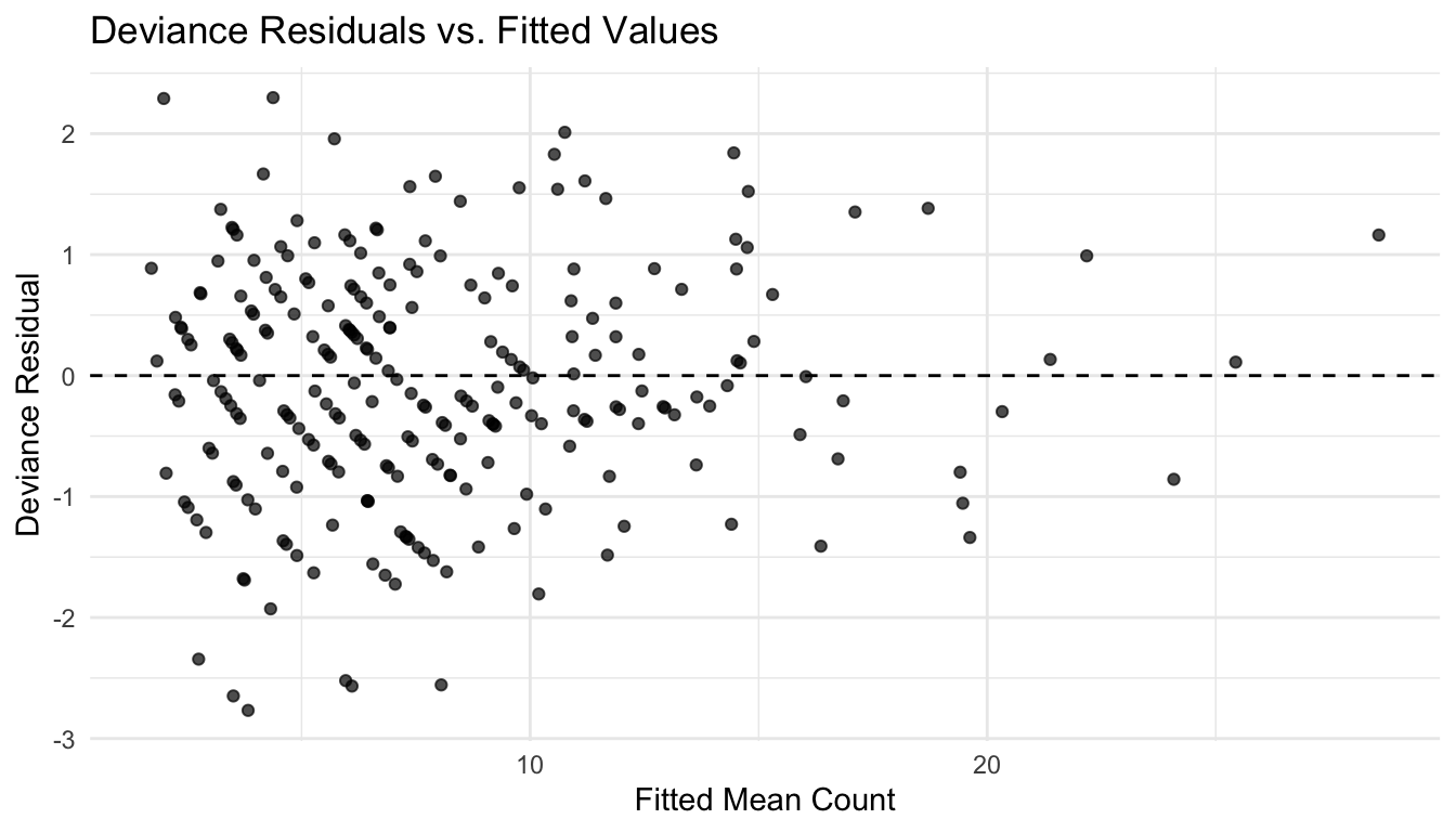
Residual Diagnostics Still Matter in GLMs

GLMs do not use all the same diagnostics as ordinary linear regression, but model checking still matters.

For example, we can inspect deviance residuals versus fitted values.

epi_df <- epi_df |>
  dplyr::mutate(
    fitted_cases = fitted(fit_pois),
    dev_resid = resid(fit_pois, type = "deviance")
  )

ggplot2::ggplot(epi_df, ggplot2::aes(x = fitted_cases, y = dev_resid)) +
  ggplot2::geom_point(alpha = 0.7) +
  ggplot2::geom_hline(yintercept = 0, linetype = 2) +
  ggplot2::labs(
    title = "Deviance Residuals vs. Fitted Values",
    x = "Fitted Mean Count",
    y = "Deviance Residual"
  ) +
  ggplot2::theme_minimal()

No diagnostic plot is perfect, but graphical checks still help reveal lack of fit, outliers, and misspecification.

GLMs Matter in AI/ML Because Real Outcomes Are Often Not Gaussian

One of the reasons GLMs remain so important in ML is that many applied outcomes are not continuous and normally distributed.

Instead, real-world ML pipelines often involve:

binary classification targets,
count-based targets,
event-rate prediction,
grouped proportions,
or skewed positive outcomes.

GLMs provide a principled way to model these outcomes while preserving:

interpretable coefficients,
link-based transformations,
and likelihood-based estimation.

This makes them especially valuable as baseline models, interpretable comparators, or production-grade models when transparency matters.

GLMs Are the Foundation for Many More Flexible Models

GLMs are not the end of the modeling story.

They are the starting point for many more advanced frameworks, including:

generalized additive models (GAMs),
mixed-effects GLMs,
negative binomial models,
zero-inflated count models,
Bayesian GLMs,
and parts of deep probabilistic architectures.

That is one reason they matter so much conceptually.

Once the analyst understands:

outcome distribution,
link function,
and linear predictor,

many later models become easier to understand.

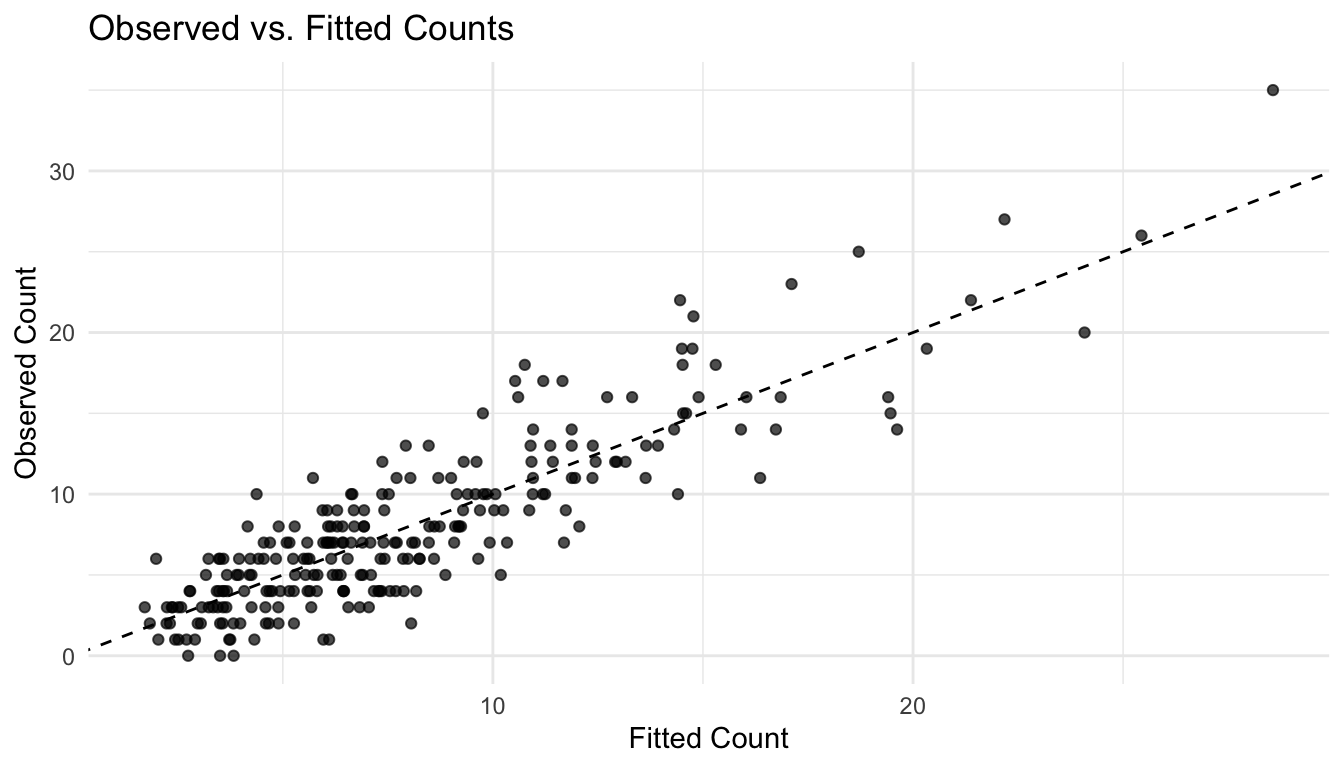
A Small Comparison of Observed and Fitted Counts

A simple plot can help readers see how the Poisson GLM behaves.

ggplot2::ggplot(epi_df, ggplot2::aes(x = fitted_cases, y = cases)) +
  ggplot2::geom_point(alpha = 0.7) +
  ggplot2::geom_abline(slope = 1, intercept = 0, linetype = 2) +
  ggplot2::labs(
    title = "Observed vs. Fitted Counts",
    x = "Fitted Count",
    y = "Observed Count"
  ) +
  ggplot2::theme_minimal()

This is not a full goodness-of-fit assessment, but it gives a quick visual sense of whether the model is capturing the count scale reasonably well.

GLMs Are Often Better Baselines Than More Complex Models

In modern ML, it is easy to reach quickly for flexible nonlinear models.

But well-specified GLMs are often strong baselines because they are:

fast,
interpretable,
probabilistic,
and tailored to the outcome type.

A Poisson GLM may outperform a poorly tuned black-box regressor on count data. A binomial GLM may provide more transparent and operationally useful risk estimates than a more complex classifier.

This is why GLMs still deserve a prominent place in both biostatistics and machine learning practice.

A Practical Checklist for Applied Work

Before fitting or reporting a GLM, ask:

What is the outcome type?
Does the chosen distribution match the data-generating structure reasonably well?
Is the link function appropriate and interpretable?
Am I modeling a count, a rate, a probability, or something else?
Is an offset needed?
Have I checked for overdispersion?
Are the coefficients being interpreted on the correct scale?
Would a more flexible extension be justified, or is the GLM already adequate?

These questions often matter more than simply whether the model converged.

Where This Shows Up in AI/ML

Poisson GLMs are the backbone of military medical surveillance: the Defense Medical Surveillance System uses rate-based models to detect excess adverse event counts across MTFs, controlling for exposure person-time via offsets. When analysts use standard linear regression instead of a Poisson GLM for count outcomes, they can produce negative predicted event rates and structurally incorrect variance estimates — both of which corrupt downstream quality improvement decisions. Negative binomial models become essential for rare trauma complications like post-traumatic osteomyelitis in penetrating injury cohorts, where overdispersion from heterogeneous facility-level reporting makes Poisson assumptions untenable. The choice of link function is not a technical detail; it encodes clinical assumptions about whether injury risk accumulates additively or multiplicatively.

Closing: GLMs Make Regression Useful for Real Data

Generalized linear models are powerful because they preserve the core strengths of regression while adapting to more realistic outcome types.

They allow analysts to move beyond normality without abandoning interpretability, likelihood-based estimation, or the logic of linear predictors.

That is why they remain so central in:

epidemiology,
biostatistics,
public health surveillance,
operational analytics,
and machine learning pipelines.

GLMs matter because the real world rarely hands us neat Gaussian outcomes, and good models must adapt to the structure of the response, not force the response into the wrong model.

📚 Go Deeper: Prediction Modeling Toolkit

This post is part of the Prediction Modeling Toolkit — a companion reference with GLM specification templates, link function selection guidance, overdispersion diagnostics, and rate-ratio reporting scaffolds.

→ Open the Prediction Modeling Toolkit

Series Callout

Note

This post is part of a broader Applied Statistics for AI and Clinical Decision-Making Series:

Probability fundamentals for machine learning
Random variables and expectation
Common probability distributions
Central Limit Theorem
Law of Large Numbers
Sampling methods for Biostats and ML
Hypothesis testing in the age of AI
Confidence intervals
Maximum likelihood estimation
Bayesian inference
Linear regression
Logistic regression
Generalized linear models
Analysis of variance
Principal component analysis
Cluster analysis
Time series analysis
Survival analysis
Non-parametric methods
Bias-variance tradeoff
Regularization
Cross-validation
Information theory
Optimization techniques
Linear algebra basics
Calculus for ML
Monte Carlo methods
Dimensionality curse and reduction techniques
Model evaluation metrics
Ensemble methods

Series: Applied Statistics for AI & Clinical Decision-Making

← Logistic Regression: Predicting Yes/No in AI and Beyond | ANOVA in ML: Uncovering Group Differences for Better Predictions →

References

Hastie, Trevor, Robert Tibshirani, and Jerome Friedman. 2009. The Elements of Statistical Learning: Data Mining, Inference, and Prediction. 2nd ed. Springer.

James, Gareth, Daniela Witten, Trevor Hastie, and Robert Tibshirani. 2021. An Introduction to Statistical Learning: With Applications in R. 2nd ed. Springer.

McCullagh, Peter, and John A. Nelder. 1989. Generalized Linear Models. 2nd ed. Chapman; Hall.

Nelder, John A., and Robert W. M. Wedderburn. 1972. “Generalized Linear Models.” Journal of the Royal Statistical Society. Series A (General) 135 (3): 370–84. https://doi.org/10.2307/2344614.