ANOVA in ML: Uncovering Group Differences for Better Predictions
Applied Statistics
Analysis of Variance
An applied introduction to ANOVA, F-statistics, one-way and two-way designs, post-hoc testing, and the connection between variance partitioning and linear models.
Published
April 15, 2024
Modified
June 9, 2026
Executive Summary
Analysis of Variance, or ANOVA, is often introduced as a method for comparing means across groups.
That is true, but incomplete.
ANOVA is really about partitioning variability.
It asks whether the variation between groups is large enough, relative to the variation within groups, to support the conclusion that group membership matters.
That idea is foundational in statistics, but it is also highly relevant in machine learning (Fisher 1925; James et al. 2021).
In classical settings, ANOVA helps answer questions like:
do treatment groups differ?
do site-level means differ?
is there an interaction between two design factors?
In AI/ML settings, the same logic appears in:
feature screening,
model comparison,
variance decomposition,
and split selection in tree-based methods.
This post introduces:
one-way ANOVA,
two-way ANOVA,
F-statistics,
post-hoc testing,
and the connection between ANOVA and linear models.
ANOVA is not just a test of group means. It is a structured way to ask whether explained variation is large relative to unexplained variation.
ANOVA Begins with Variability, Not Just Means
At a surface level, ANOVA compares group means.
At a deeper level, it compares two sources of variation:
variation between groups
variation within groups
If the between-group variation is large relative to the within-group variation, that suggests the grouping variable helps explain the outcome.
This is why ANOVA is built around the F-statistic:
\[
F = \frac{\text{Mean Square Between}}{\text{Mean Square Within}}
\]
A large F-value suggests that group membership explains more variability than would be expected from random within-group fluctuation alone.
For example, we might ask whether average follow-up time differs across three treatment groups.
We will simulate a simple biostats-style example.
library(dplyr)library(tibble)library(ggplot2)oneway_df <- tibble::tibble(treatment =rep(c("Standard", "Enhanced", "Intensive"), each =50),outcome =c(rnorm(50, mean =12, sd =3),rnorm(50, mean =14, sd =3),rnorm(50, mean =16, sd =3) ))oneway_df |> dplyr::group_by(treatment) |> dplyr::summarise(n = dplyr::n(),mean =mean(outcome),sd =sd(outcome),.groups ="drop" )
# A tibble: 3 × 4
  treatment     n  mean    sd
  <chr>     <int> <dbl> <dbl>
1 Enhanced     50  14.1  2.92
2 Intensive    50  15.9  3.14
3 Standard     50  11.8  3.41
Now fit the one-way ANOVA.
fit_oneway <-aov(outcome ~ treatment, data = oneway_df)summary(fit_oneway)
             Df Sum Sq Mean Sq F value   Pr(>F)
treatment     2    422     211    21.1 8.77e-09 ***
Residuals   147   1470      10
---
Signif. codes:  0 '***' 0.001 '**' 0.01 '*' 0.05 '.' 0.1 ' ' 1
This ANOVA table shows whether the treatment factor explains a significant portion of the variability in outcome.
The F-Statistic Compares Signal to Noise
The F-statistic is often presented mechanically, but conceptually it is simple.
It asks:
is the variation across group means large compared with the ordinary variation among individuals inside those groups?
If yes, that supports the idea that the grouping factor matters.
If no, then the group means may differ only by the kind of fluctuation we would expect even if the population means were the same.
This is why ANOVA is fundamentally about signal relative to noise.
That same basic logic appears all over machine learning.
Visualization Helps Before Formal Testing
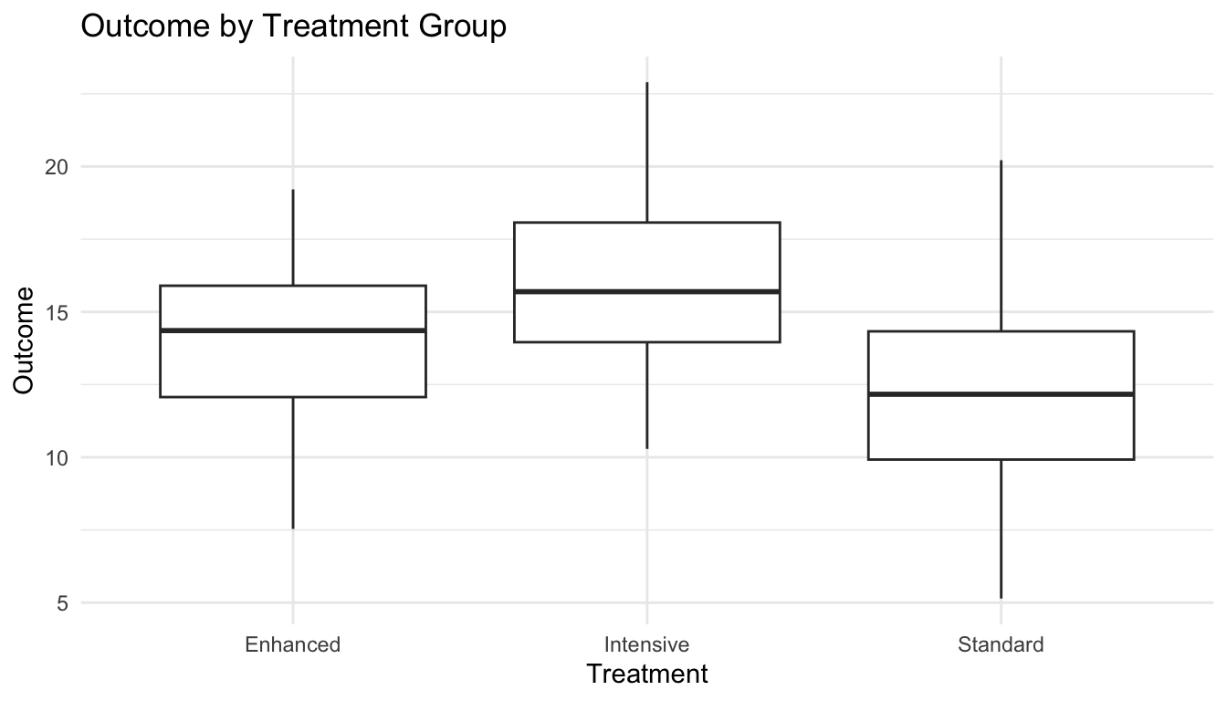
As with most models, it helps to visualize the data before interpreting the ANOVA table.
ggplot2::ggplot(oneway_df, ggplot2::aes(x = treatment, y = outcome)) + ggplot2::geom_boxplot() + ggplot2::labs(title ="Outcome by Treatment Group",x ="Treatment",y ="Outcome" ) + ggplot2::theme_minimal()
A plot helps reveal:
group separation,
spread,
outliers,
and overlap.
That context matters because ANOVA can tell us a difference exists without showing us the pattern of that difference clearly.
ANOVA and Linear Regression Are Closely Connected
One of the most important conceptual points about ANOVA is that it is not separate from regression.
ANOVA is a special case of the general linear model.
A one-way ANOVA can be written as a regression model using indicator variables for group membership.
That means:
the ANOVA table,
sums of squares,
F-tests,
and regression-based model comparison
are all closely related.
This matters because it unifies statistical thinking.
Instead of viewing ANOVA and regression as separate topics, it is better to see them as different presentations of the same underlying model structure.
ANOVA Assumptions Still Matter
Classical ANOVA relies on assumptions similar to those of linear models.
The main ones are:
independence of observations
approximate normality of residuals
homogeneity of variance across groups
These assumptions do not have to be perfect, but large violations can affect the validity of the F-test and its interpretation.
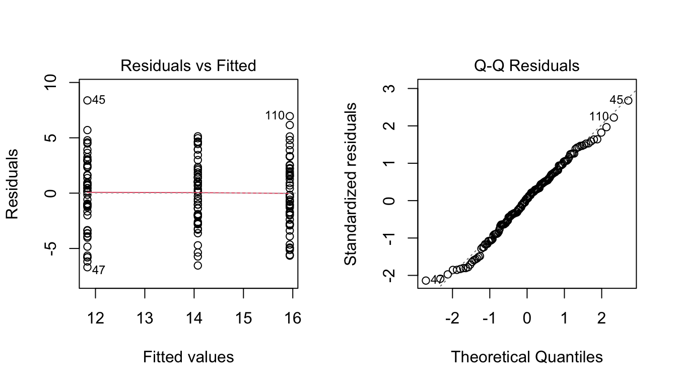
We can inspect basic diagnostics.
par(mfrow =c(1, 2))plot(fit_oneway, which =1)plot(fit_oneway, which =2)
par(mfrow =c(1, 1))
These plots help assess:
residual spread versus fitted values
approximate residual normality
In applied work, the goal is not perfection. It is to determine whether the model is grossly inconsistent with the data.
A Significant ANOVA Does Not Tell You Which Groups Differ
A common misunderstanding is that a significant one-way ANOVA tells us exactly which groups differ.
It does not.
It only tells us that at least one group mean differs from at least one other.
That is why post-hoc testing is needed when there are multiple groups.
A common approach is Tukey’s Honest Significant Difference procedure.
TukeyHSD(fit_oneway)
  Tukey multiple comparisons of means
    95% family-wise confidence level

Fit: aov(formula = outcome ~ treatment, data = oneway_df)

$treatment
                        diff        lwr        upr     p adj
Intensive-Enhanced  1.863729  0.3664055  3.3610522 0.0103706
Standard-Enhanced  -2.238977 -3.7363004 -0.7416536 0.0015445
Standard-Intensive -4.102706 -5.6000292 -2.6053825 0.0000000
This provides pairwise comparisons while accounting for multiple testing.
That is often much more informative than the overall omnibus F-test alone.
Post-Hoc Testing Helps Translate the Omnibus Result
The omnibus ANOVA answers:
is there evidence of any group difference at all?
Post-hoc tests answer:
where are the differences?
This distinction matters because scientific or operational decisions usually depend on specific comparisons, not just the existence of some overall heterogeneity.
For example:
is Intensive different from Standard?
is Enhanced different from Standard?
are Enhanced and Intensive practically similar?
The ANOVA table opens the door. Post-hoc analysis tells the more actionable story.
Two-Way ANOVA Adds a Second Factor
A two-way ANOVA is used when there are:
two categorical predictors
and one continuous outcome
This allows us to study:
the main effect of factor A
the main effect of factor B
and their interaction
A factorial design is one of the most useful settings for seeing this clearly.
We will simulate a simple example with:
treatment group
and sex
affecting a continuous response
twoway_df <-expand.grid(treatment =c("Standard", "Enhanced"),sex =c("Female", "Male"),rep =1:40) |> tibble::as_tibble() |> dplyr::mutate(outcome = dplyr::case_when( treatment =="Standard"& sex =="Female"~rnorm(dplyr::n(), mean =10, sd =2.5), treatment =="Standard"& sex =="Male"~rnorm(dplyr::n(), mean =11, sd =2.5), treatment =="Enhanced"& sex =="Female"~rnorm(dplyr::n(), mean =13, sd =2.5), treatment =="Enhanced"& sex =="Male"~rnorm(dplyr::n(), mean =16, sd =2.5),TRUE~NA_real_ ) )twoway_df |> dplyr::group_by(treatment, sex) |> dplyr::summarise(mean =mean(outcome),sd =sd(outcome),.groups ="drop" )
# A tibble: 4 × 4
  treatment sex     mean    sd
  <fct>     <fct>  <dbl> <dbl>
1 Standard  Female  10.2  2.18
2 Standard  Male    10.6  2.81
3 Enhanced  Female  12.3  2.86
4 Enhanced  Male    16.0  1.96
Now fit the two-way ANOVA.
fit_twoway <-aov(outcome ~ treatment * sex, data = twoway_df)summary(fit_twoway)
               Df Sum Sq Mean Sq F value   Pr(>F)
treatment       1  570.9   570.9   92.50  < 2e-16 ***
sex             1  171.1   171.1   27.72 4.57e-07 ***
treatment:sex   1  101.1   101.1   16.38 8.12e-05 ***
Residuals     156  962.8     6.2
---
Signif. codes:  0 '***' 0.001 '**' 0.01 '*' 0.05 '.' 0.1 ' ' 1
The treatment * sex term includes both main effects and the interaction.
Interactions Are Often the Most Important Part
A main effect tells us whether one factor matters on average across the levels of the other factor.
An interaction tells us whether the effect of one factor depends on the level of the other.
That is often where the most interesting scientific story lies.
For example:
treatment may work differently in different subgroups
interventions may be more effective under one condition than another
group differences may not be constant across design cells
This is one reason factorial ANOVA is so useful.
It forces us to ask whether effects are additive or conditional.
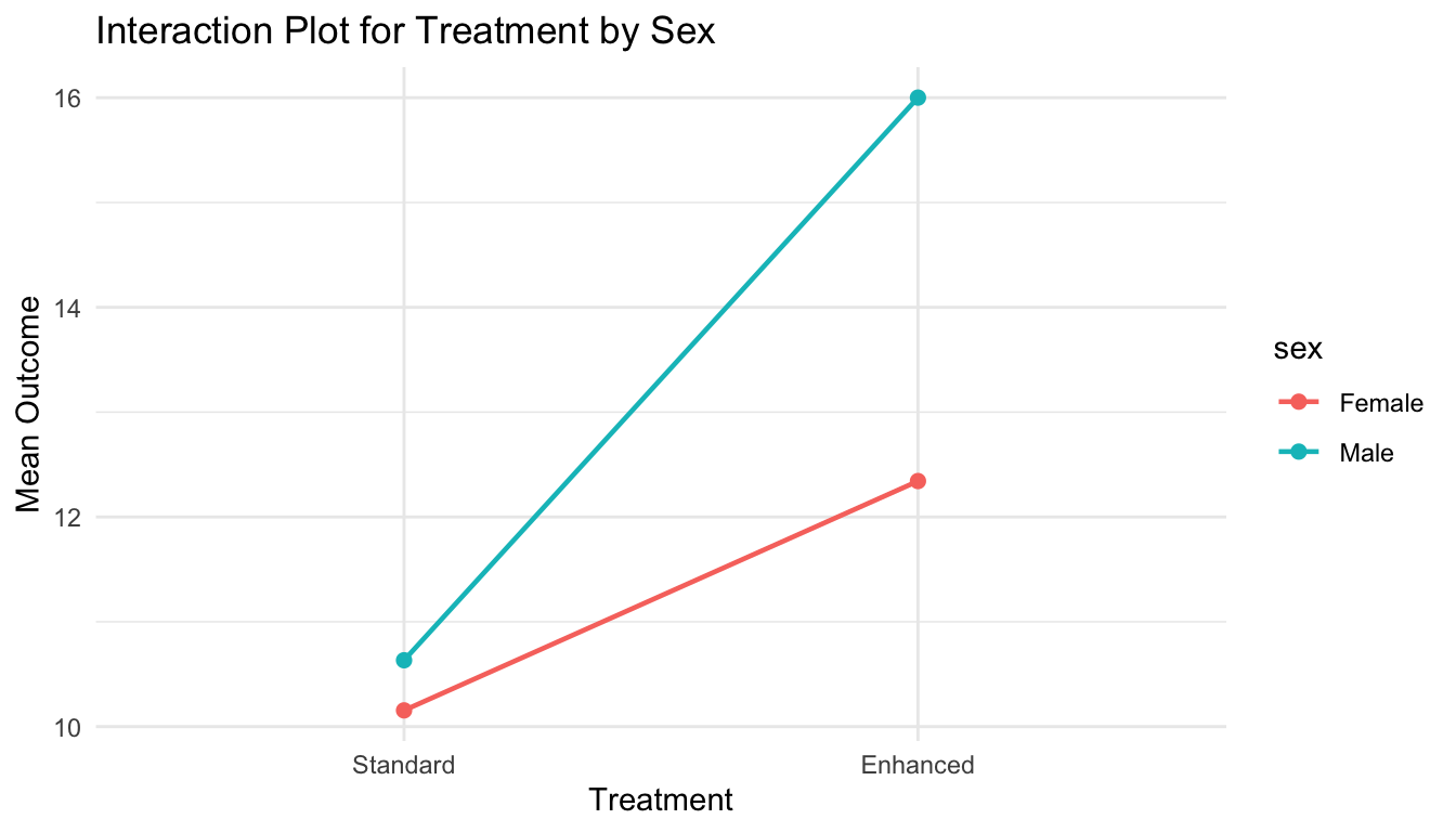
Interaction Plots Make Two-Way ANOVA More Intuitive
Interaction tables can be abstract. A plot often makes the interpretation much clearer.
ggplot2::ggplot( twoway_df, ggplot2::aes(x = treatment, y = outcome, color = sex, group = sex)) + ggplot2::stat_summary(fun = mean, geom ="point", size =2) + ggplot2::stat_summary(fun = mean, geom ="line", linewidth =0.8) + ggplot2::labs(title ="Interaction Plot for Treatment by Sex",x ="Treatment",y ="Mean Outcome" ) + ggplot2::theme_minimal()
If the lines are roughly parallel, the interaction may be small. If the lines diverge or cross, the interaction may be substantial.
This is often much easier to explain to readers than the raw ANOVA table alone.
ANOVA Is Really About Sums of Squares
A classic ANOVA table partitions total variability into components.
It shows how total variability can be divided into interpretable parts.
That same logic reappears in many forms of model evaluation and variable importance thinking.
ANOVA Connects Naturally to Feature Screening in ML
Although ML workflows often do not rely on classical ANOVA tables directly, the logic still appears.
For example, ANOVA-style reasoning can be used in:
univariate feature screening,
comparing mean response across categories,
evaluating whether a predictor explains meaningful variation,
and ranking variables by explained variance.
This is especially common in preprocessing or exploratory analysis.
A variable that explains very little group-based variation may contribute less signal, while one associated with substantial variance partitioning may warrant further modeling attention.
Of course, univariate screening is not the whole story. But ANOVA remains a useful lens.
Tree-Based Models Also Partition Variance
One reason ANOVA remains relevant in AI/ML is that its logic resembles what happens in tree-based methods.
Decision trees and ensembles such as random forests often split variables based on impurity reduction or error reduction.
That is not identical to classical ANOVA, but conceptually it is related:
identify splits
reduce unexplained variation
improve group separation
So ANOVA can be viewed as part of the broader family of variance-partitioning ideas that still matter in modern predictive systems.
Model Comparison Can Also Be Framed in ANOVA Terms
Because ANOVA is part of the general linear model framework, it can be used for nested model comparison.
For example, we can compare whether adding a factor improves fit relative to a simpler model.
fit_null <-lm(outcome ~1, data = oneway_df)fit_factor <-lm(outcome ~ treatment, data = oneway_df)anova(fit_null, fit_factor)
Analysis of Variance Table

Model 1: outcome ~ 1
Model 2: outcome ~ treatment
  Res.Df    RSS Df Sum of Sq      F    Pr(>F)
1    149 1891.7
2    147 1469.7  2    421.98 21.103 8.774e-09 ***
---
Signif. codes:  0 '***' 0.001 '**' 0.01 '*' 0.05 '.' 0.1 ' ' 1
This is another reminder that ANOVA is not only about textbook group comparisons. It is also a general framework for comparing explained variability across nested models.
As with many classical tests, ANOVA results are often over-reduced to whether the p-value is below 0.05.
That is not enough.
It is also useful to think about effect size.
One simple descriptive summary is the group means themselves. Another is a measure such as eta-squared, which reflects the proportion of total variance explained by the factor.
how much of the variability does the grouping factor actually explain?
That is usually a better question.
ANOVA Is Useful, but It Does Not Fix Bad Design
ANOVA is powerful, but like any method, it depends on the quality of the design and data.
It cannot rescue:
poor sampling,
uncontrolled confounding,
measurement error,
dependence among observations,
or post-hoc subgroup fishing.
A clean ANOVA table may still reflect a weak study design.
This is especially important in both biostatistics and ML, where statistical significance can create false confidence if the underlying data structure is flawed.
A Practical Checklist for Applied Work
Before reporting an ANOVA, ask:
Is the outcome continuous enough for ANOVA to be reasonable?
Are the grouping variables clearly defined?
Is the design one-way or factorial?
Have I checked approximate variance homogeneity and residual behavior?
If the omnibus test is significant, have I followed with the right post-hoc comparisons?
Is interaction more important than the main effects?
Am I interpreting effect size, not just p-values?
Would a regression framing communicate the result more clearly?
These questions usually improve both rigor and explanation.
NoteWhere This Shows Up in AI/ML
ANOVA is the statistical engine behind clinical AI A/B testing: when a health system compares model version 2.1 against 2.0 across patient subgroups, the test of whether outcome differences exceed random within-group variation is structurally identical to a factorial ANOVA. In fairness auditing, subgroup performance analysis across demographic groups — required by FDA guidance on AI/ML-based software as a medical device — is essentially an ANOVA-framed question: does model AUC or calibration error differ significantly across race, sex, or age strata beyond what chance variation would produce? When this analysis is skipped or underpowered, models that perform acceptably on average can embed substantial disparities in care quality across MTF locations or patient populations. Interaction effects matter most here — a model that performs well for combat-injured males may perform poorly for female service members with the same injury pattern, a gap that main-effect analysis alone cannot detect.
Closing: ANOVA Still Teaches a Core Modeling Idea
ANOVA remains important because it teaches one of the deepest ideas in applied statistics:
variation can be partitioned into meaningful components.
That idea matters in:
treatment comparisons,
factorial experiments,
model comparison,
feature screening,
and even tree-based learning.
One-way ANOVA helps compare groups. Two-way ANOVA helps reveal interactions. Post-hoc testing clarifies where the differences lie. And the connection to linear models helps unify these ideas into a broader modeling framework.
ANOVA still matters because the question “what explains variability?” remains central in both statistics and machine learning.
This post is part of the Trauma Registry Analytics Toolkit — a companion reference with multi-site comparison templates, post-hoc testing code, effect size reporting, and reviewer-ready ANOVA language for registry analyses.
Fisher, Ronald A. 1925. Statistical Methods for Research Workers. Oliver; Boyd.
James, Gareth, Daniela Witten, Trevor Hastie, and Robert Tibshirani. 2021. An Introduction to Statistical Learning: With Applications in R. 2nd ed. Springer.