Identification Strategies: IV, DAGs & Target Trial Emulation

Advanced Statistics for AI & Clinical Decision-Making — Lecture 3 of 4

Jonathan D. Stallings, PhD, MS

Data InDeed | dataindeed.org

2026-01-01

When adjustment isn’t enough — three strategies for causal identification in the hardest observational settings.

What You’ll Learn Today

Post 06 Instrumental Variables

  • The endogeneity problem
  • Three IV assumptions
  • Two-stage least squares
  • Weak instrument danger

Post 07 DAGs & Confounding

  • Graphical causal reasoning
  • Forks, chains, colliders
  • What not to adjust for
  • E-values and sensitivity

Post 08 Target Trial Emulation

  • Define the trial you’d want
  • Time zero, eligibility, estimand
  • G-computation
  • Common pitfalls

Part 1

Instrumental Variables

Causal identification when unmeasured confounding is unavoidable

When Propensity Scores Break Down

Propensity scores balance measured confounders.

If an important confounder is unmeasured, the treatment-outcome relationship remains biased — no matter how good the propensity model is.

Endogeneity: Treatment \(A\) is correlated with the error term in the outcome model.

\[Y = \alpha + \beta A + \gamma X + \underbrace{(\delta U + \varepsilon)}_{\text{error includes }U}\]

If \(U\) causes both \(A\) and \(Y\), OLS estimate of \(\beta\) is biased.

Solution: Find a variable \(Z\) that moves \(A\) but is unrelated to \(U\) or \(Y\) except through \(A\).

Trauma example:

Surgeon preference for DCS vs. definitive surgery.

Surgeons on call at 0300 may default to DCS more often — but this “instrument” is unrelated to patient severity (the unmeasured confounder).

Distance to trauma center: affects care received, unrelated to injury mechanism.

The Three IV Assumptions

A valid instrument \(Z\) must satisfy:

  1. Relevance: \(Z\) causally affects treatment \(A\) — testable via F-statistic
  2. Exclusion restriction: \(Z\) affects outcome \(Y\) only through \(A\) — not directly
  3. Independence: \(Z\) is independent of unmeasured confounders \(U\) — not directly testable

The weak instrument problem: If \(Z\) barely predicts \(A\) (F < 10 in first stage), 2SLS estimates are nearly as biased as OLS, but with much larger standard errors. A weak instrument is worse than no instrument.

Two-Stage Least Squares

n <- 500
# U = unmeasured confounder (patient frailty)
U <- rnorm(n)
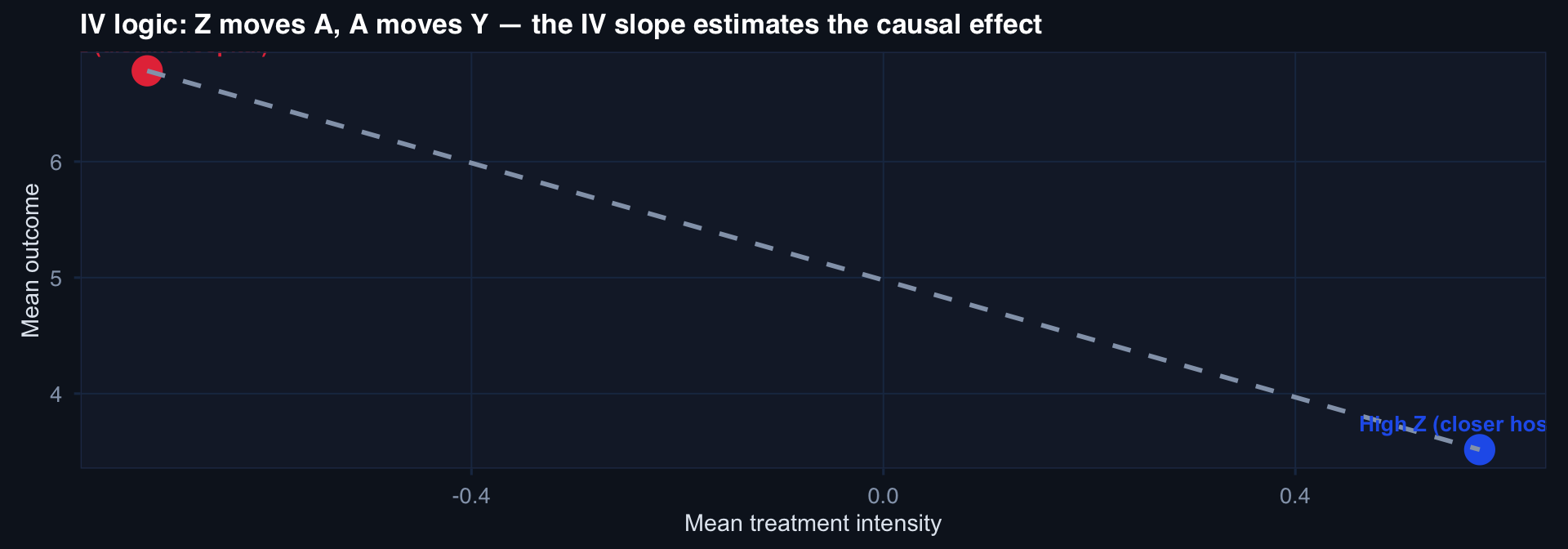
# Z = instrument (hospital distance, affects care but not frailty)
Z <- rnorm(n)
# Treatment (DCS): driven by U and Z
A <- 0.8*Z - 1.2*U + rnorm(n, 0, 0.8)
# Outcome: true treatment effect = -2, U also worsens outcome
Y <- 5 - 2*A + 2.5*U + rnorm(n, 0, 2)

# OLS (biased)
ols_est <- coef(lm(Y ~ A))["A"]

# 2SLS manually
stage1 <- lm(A ~ Z)
A_hat  <- fitted(stage1)
stage2 <- lm(Y ~ A_hat)
iv_est <- coef(stage2)["A_hat"]

# First-stage F
f_stat <- summary(stage1)$fstatistic[1]

tibble(
  Method    = c("OLS (biased)", "2SLS (IV)", "True effect"),
  Estimate  = round(c(ols_est, iv_est, -2), 3),
  `F-stat`  = c(NA, round(f_stat, 1), NA)
)
# A tibble: 3 × 3
  Method       Estimate `F-stat`
  <chr>           <dbl>    <dbl>
1 OLS (biased)    -3.12      NA 
2 2SLS (IV)       -2.45     197.
3 True effect     -2         NA 

Visualizing the IV Logic

tibble(Z=Z, A=A, Y=Y) |>
  mutate(Z_group = ifelse(Z > 0, "High Z (closer hospital)", "Low Z (distant hospital)")) |>
  group_by(Z_group) |>
  summarise(mean_A = mean(A), mean_Y = mean(Y), .groups="drop") |>
  ggplot(aes(mean_A, mean_Y, color=Z_group, label=Z_group)) +
  geom_point(size=6) +
  geom_line(aes(group=1), color="#94a3b8", linewidth=1, linetype=2) +
  ggplot2::geom_text(vjust=-1.2, size=3.5, fontface="bold") +
  scale_color_manual(values=c("#2563eb","#e63946")) +
  labs(title="IV logic: Z moves A, A moves Y — the IV slope estimates the causal effect",
       x="Mean treatment intensity", y="Mean outcome", color=NULL) +
  theme_di() + theme(legend.position="none")

Wald estimator: \(\hat\beta_{IV} = \frac{\text{Cov}(Z,Y)}{\text{Cov}(Z,A)}\) — the reduced-form slope divided by the first-stage slope.

Part 2

DAGs & Confounding

Drawing causation before modeling it

Directed Acyclic Graphs: The Causal Language

Three fundamental structures determine what you should and shouldn’t adjust for:

Fork (common cause)

U → A
U → Y

\(U\) confounds \(A\)\(Y\). Adjust for \(U\) to block the backdoor path.

Chain (mediation)

A → M → Y

\(M\) mediates \(A\)\(Y\). Don’t adjust for \(M\) if you want the total effect.

Collider (selection)

A → C ← Y

\(C\) is a collider. Never adjust for \(C\) — conditioning on a collider opens a spurious path.

Collider bias in trauma registries: Conditioning on “survived to hospital” (a collider of injury severity and treatment quality) induces a spurious correlation between severity and treatment. This is survivorship bias reframed as a DAG.

E-Values: Quantifying Unmeasured Confounding

# E-value: minimum confounding association needed to explain away a result
# For a risk ratio RR:
evalue <- function(RR) RR + sqrt(RR * (RR - 1))

rr_grid <- seq(1.05, 4, by=0.05)
tibble(RR=rr_grid, Evalue=evalue(rr_grid)) |>
  ggplot(aes(RR, Evalue)) +
  geom_line(linewidth=1.4, color="#0891b2") +
  geom_hline(yintercept=2, linetype=2, color="#e63946", linewidth=0.8) +
  annotate("text", x=3.5, y=2.15, label="E-value = 2\n(moderate robustness)",
           color="#e63946", size=3.2) +
  labs(title="E-value by observed risk ratio — higher = more robust to unmeasured confounding",
       x="Observed Risk Ratio", y="E-value") + theme_di()

Interpretation: An E-value of 3.0 means an unmeasured confounder would need to be associated with both treatment and outcome by a risk ratio of at least 3.0 to fully explain away the result. Clinically plausible?

Standardization: The Explicit G-Formula

n <- 600
df_std <- tibble(
  confounder = rbinom(n, 1, 0.5),      # e.g., penetrating mechanism
  treated    = rbinom(n, 1, plogis(-0.5 + 1.5*confounder)),
  outcome    = 3 - 1.8*treated + 2*confounder + rnorm(n, 0, 2)
)

# Standardization (g-computation for continuous outcome)
# Step 1: fit outcome model
fit <- lm(outcome ~ treated + confounder, data=df_std)

# Step 2: predict potential outcomes for everyone
po1 <- predict(fit, newdata=mutate(df_std, treated=1))
po0 <- predict(fit, newdata=mutate(df_std, treated=0))

cat("Naive (unadjusted) effect: ", round(mean(df_std$outcome[df_std$treated==1]) -
                                          mean(df_std$outcome[df_std$treated==0]), 3))
Naive (unadjusted) effect:  -1.19
cat("\nStandardized ATE:         ", round(mean(po1 - po0), 3))

Standardized ATE:          -1.833
cat("\nTrue ATE:                  -1.8")

True ATE:                  -1.8

Standardization answers: “What would the population mean outcome be if everyone were treated vs. untreated?” — the population-level causal question, not the conditional association.

Part 3

Target Trial Emulation

Designing observational studies as if they were trials

The Target Trial Framework

Most observational studies fail not because of statistics — but because of design ambiguity.

Hernán & Robins: Before any analysis of observational data, write down the randomized trial you would conduct if you could. Then emulate it exactly.

Trial component Must be specified
Eligibility Who enters? At what time?
Treatment strategies What interventions are compared?
Time zero When does follow-up begin?
Outcomes What is measured? When?
Estimand Per-protocol? Intention-to-treat?
Analysis How is confounding handled?

Time Zero: The Most Common Design Failure

Immortal time bias: When follow-up begins before treatment assignment is finalized, patients who survive long enough to receive treatment appear healthier — because the dead can’t be treated.

Example: Studying antibiotic timing in trauma.

  • Wrong: time zero = hospital admission; treatment = antibiotics “at any point”
  • Right: time zero = injury; treatment strategies = “antibiotics within 1h” vs. “antibiotics after 1h”

DoDTR application:

“Early tourniquet application” studies often suffer from immortal time bias — soldiers who died before tourniquet could be applied are excluded from the “no tourniquet” group.

Time zero must be point of injury, not point of registry entry.

G-Computation for Trial Emulation

n <- 500
# Simulate observational data with time zero properly defined
df_tt <- tibble(
  severity  = rnorm(n, 30, 10),
  early_tx  = rbinom(n, 1, plogis(-1 + 0.04*severity)),  # sicker → more likely early tx
  outcome   = 15 - 3*early_tx + 0.3*severity + rnorm(n, 0, 3)
)

# G-computation (standardization)
outcome_model <- lm(outcome ~ early_tx + severity, data=df_tt)

# Estimate ATE: E[Y(1)] - E[Y(0)] standardized over population
ate_g <- mean(
  predict(outcome_model, newdata=mutate(df_tt, early_tx=1)) -
  predict(outcome_model, newdata=mutate(df_tt, early_tx=0))
)

# Compare to naive
ate_naive <- mean(df_tt$outcome[df_tt$early_tx==1]) -
             mean(df_tt$outcome[df_tt$early_tx==0])

cat("Naive comparison:  ", round(ate_naive, 3))
Naive comparison:   -2.422
cat("\nG-computation ATE: ", round(ate_g, 3))

G-computation ATE:  -2.98
cat("\nTrue ATE:          -3.0")

True ATE:          -3.0

Lecture 3 — Key Takeaways

Instrumental Variables

  • Addresses unmeasured confounding — propensity scores cannot
  • Valid instrument: relevance, exclusion, independence
  • F-statistic > 10 in first stage (weak instrument check)
  • 2SLS estimates LATE (local average treatment effect) — not ATE

DAGs & Confounding

  • Draw the DAG before fitting any model
  • Forks: adjust. Chains: don’t adjust for mediators. Colliders: never adjust
  • E-values quantify robustness to unmeasured confounding

Target Trial Emulation

  • Specify the trial before analyzing the data
  • Time zero is the most common source of bias
  • Immortal time bias is preventable by design
  • G-computation estimates the standardized population effect

The meta-lesson: These three methods exist because the confounding problem is harder than it looks. Each requires strong, untestable assumptions — the job is to state them clearly, not to hide them in the modeling choices.

Coming Up: Lecture 4

Evidence Synthesis — Meta-Analysis & Real-World Generalizability

Posts 09 & 10:

  • Meta-analysis — fixed vs. random effects, heterogeneity (I²), forest plots, Bayesian pooling
  • RWE generalizability — transportability, reweighting, site effects, model performance transport

After building a rigorous estimate from one dataset — how do you combine it with others, and does it generalize to a new population?