Dimensionality Reduction & Clustering

Applied Statistics for AI & Clinical Decision-Making — Lecture 7 of 10

Jonathan D. Stallings, PhD, MS

Data InDeed | dataindeed.org

2026-01-01

When you have 500 features and 200 patients, you don’t have a big dataset. You have a geometry problem.

What You’ll Learn Today

Post 15 PCA

• Variance decomposition
• Loadings & scores
• Scree plots

Post 16 Clustering

• k-means, hierarchical
• Choosing k
• Clinical phenotyping

Post 28 Dimensionality Curse

• Distance breakdown
• Sparsity in high-p
• Solutions

Part 1

Principal Component Analysis

Finding the directions that matter most

PCA: The Core Idea

Rotate the coordinate system so the first axis captures the most variance, the second axis (orthogonal) captures the next most, and so on.

Covariance matrix: \(\Sigma = \frac{1}{n-1}X^\top X\)

Eigen decomposition: \(\Sigma v_k = \lambda_k v_k\)

PC scores = \(XV\) (data projected onto eigenvectors)

Trauma phenotyping: 15 physiologic variables (HR, SBP, lactate, GCS, RR, SpO2…) reduced to 2-3 principal components that capture injury severity patterns — enabling visualization and unsupervised clustering of injury profiles.

PCA in R: Registry Example

n <- 300
df_pca <- tibble(
  sbp      = rnorm(n,110,20),
  hr       = rnorm(n,95,18),
  rr       = rnorm(n,18,4),
  gcs      = rnorm(n,13,3),
  lactate  = rexp(n, 0.5) + 1,
  spo2     = rnorm(n,96,3)
)
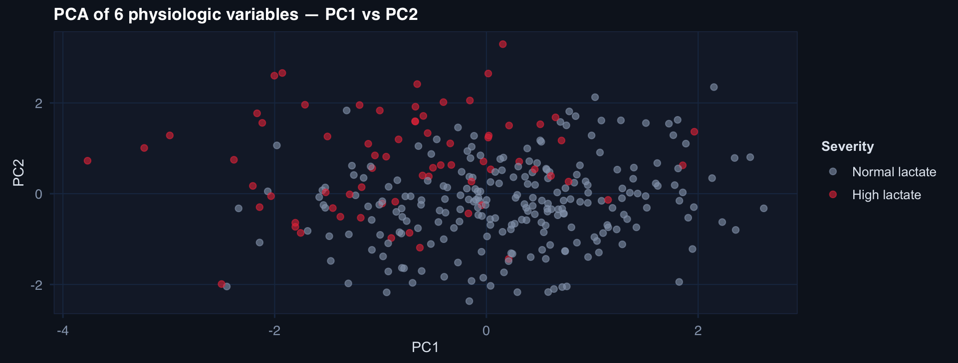
pca_fit <- prcomp(df_pca, scale.=TRUE)
pca_df  <- as_tibble(pca_fit$x[,1:2]) |>
  mutate(severity = df_pca$lactate > 4)

ggplot(pca_df, aes(PC1, PC2, color=severity)) +
  geom_point(alpha=0.6) +
  scale_color_manual(values=c("FALSE"="#94a3b8","TRUE"="#e63946"),
                     labels=c("Normal lactate","High lactate")) +
  labs(title="PCA of 6 physiologic variables — PC1 vs PC2",
       color="Severity") + theme_di()

Scree Plot: How Many Components?

var_explained <- pca_fit$sdev^2 / sum(pca_fit$sdev^2)
tibble(PC = paste0("PC",1:6), pct = var_explained * 100) |>
  ggplot(aes(x=PC, y=pct, group=1)) +
  geom_col(fill="#2563eb", alpha=0.8) +
  geom_line(linewidth=1, color="#1b2e4b") +
  geom_point(size=3, color="#1b2e4b") +
  labs(title="Scree plot: variance explained by each PC",
       x="Principal Component", y="% Variance Explained") + theme_di()

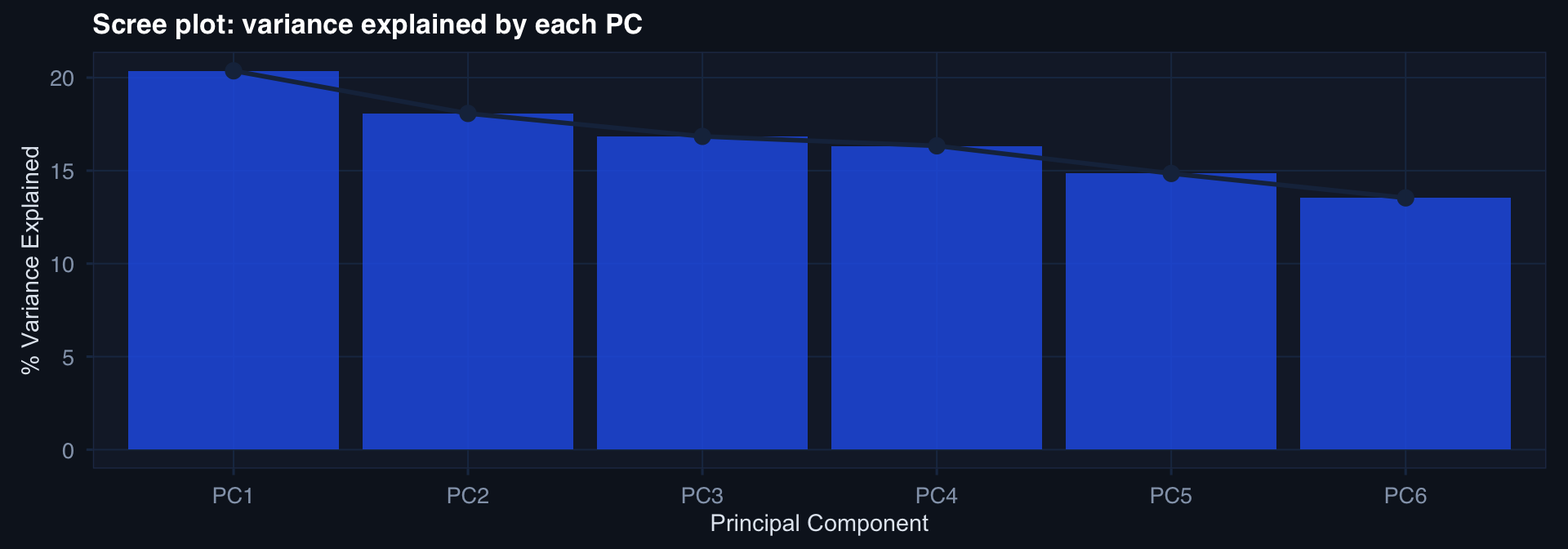
Practical rule: retain PCs until you explain ~80% of variance, or where the scree “elbows.”

Part 2

Clustering

Grouping patients without labels

k-Means: Partitioning by Centroid Distance

Minimize: \(\sum_{k=1}^K \sum_{i \in C_k} \| x_i - \mu_k \|^2\)

km <- kmeans(df_pca, centers=3, nstart=20)
df_pca |>
  mutate(cluster = factor(km$cluster)) |>
  ggplot(aes(sbp, lactate, color=cluster)) +
  geom_point(alpha=0.6) +
  scale_color_manual(values=c("#2563eb","#e63946","#0891b2")) +
  labs(title="k-means clustering: 3 injury phenotype groups",
       x="SBP", y="Lactate") + theme_di()

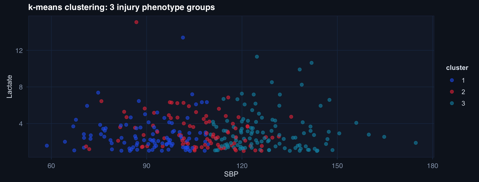
Trauma phenotyping clusters might correspond to: compensated shock (normal SBP, mild lactate elevation), uncompensated shock (low SBP, high lactate), neurological dominant injury (normal physiology, low GCS).

Choosing k: The Elbow and Silhouette

wss <- sapply(1:8, function(k) kmeans(df_pca, k, nstart=10)$tot.withinss)
tibble(k=1:8, wss=wss) |>
  ggplot(aes(k, wss)) +
  geom_line(linewidth=1.2, color="#2563eb") +
  geom_point(size=3, color="#1b2e4b") +
  geom_vline(xintercept=3, linetype=2, color="#e63946") +
  labs(title="Elbow method: within-cluster sum of squares vs. k",
       x="Number of clusters k", y="Total WSS") + theme_di()

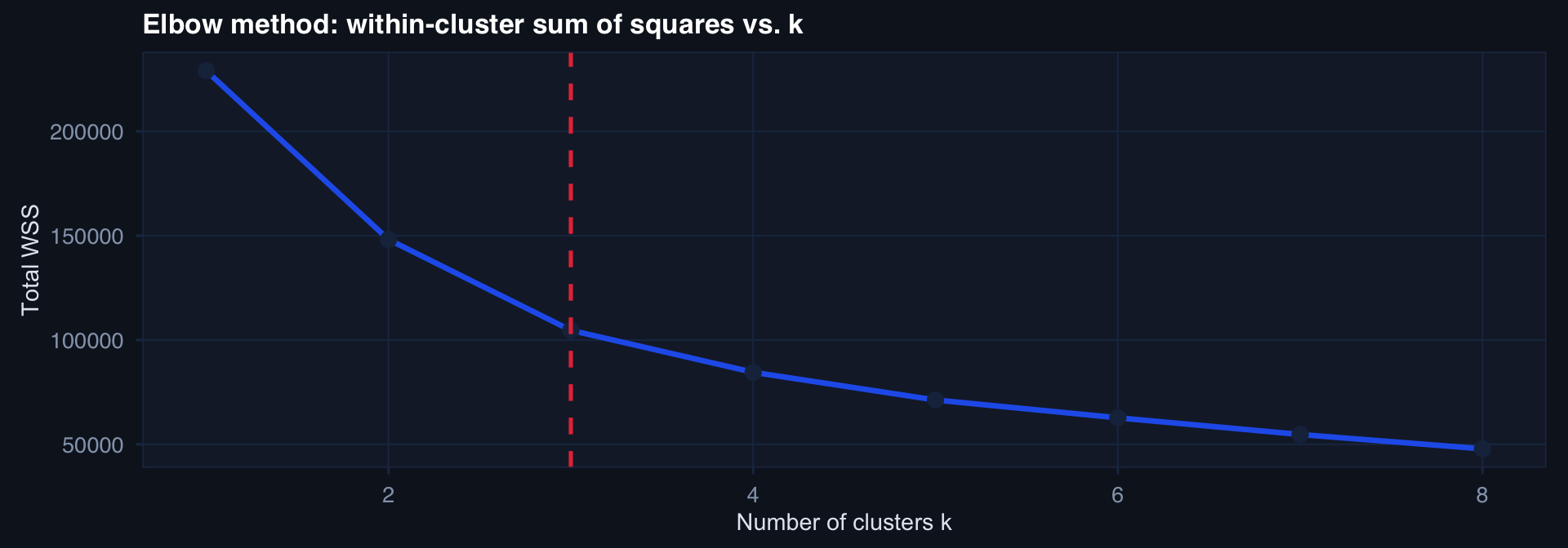
The “elbow” where WSS stops decreasing sharply suggests k=3. Validate clinically — do the clusters correspond to meaningful patient phenotypes?

Part 3

The Curse of Dimensionality

Why p >> n changes everything

Distance Breaks Down in High Dimensions

set.seed(42)
compute_dist_ratio <- function(p, n=100) {
  X <- matrix(runif(n*p), n, p)
  dists <- as.vector(dist(X))
  max(dists) / min(dists)
}

dims <- c(1,2,5,10,50,100,200,500)
ratios <- sapply(dims, compute_dist_ratio)

tibble(p=dims, ratio=ratios) |>
  ggplot(aes(p, ratio)) +
  geom_line(linewidth=1.2, color="#2563eb") +
  geom_point(size=3, color="#1b2e4b") +
  scale_x_log10() +
  labs(title="Max/min distance ratio approaches 1 as dimensions grow",
       x="Dimensions (log scale)", y="max dist / min dist") + theme_di()

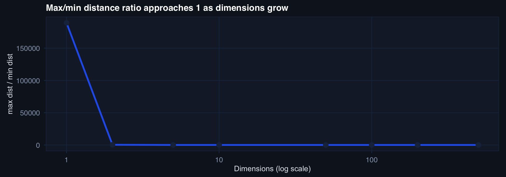
When max ≈ min distance: kNN, clustering, and distance-based models lose meaning. Every point is equidistant from every other point.

Solutions: Reduce Before You Model

Strategy 1: Feature selection

• Keep only the p variables most predictive of the outcome
• Lasso / elastic net (Lecture 8) does this automatically

Strategy 2: Dimensionality reduction

• PCA → replace p features with k components (k << p)
• Autoencoders → nonlinear compression

Strategy 3: Regularization

• Penalize coefficient magnitude → shrinks irrelevant features toward zero
• Ridge and Lasso (Lecture 8)

Strategy 4: Domain expertise

• The most underused solution in registry analytics
• Clinical knowledge about which features matter reduces effective dimensionality before any model is fit

In trauma registry work, you often have 200+ coded variables. Feeding all of them into a logistic regression is almost always a mistake. Feature selection, dimensionality reduction, or clinical domain knowledge should reduce that to 15-20 clinically meaningful features before modeling begins.

Lecture 7 — Key Takeaways

PCA

• Rotates to directions of maximum variance
• Scree plot guides component selection
• Scores = data in PC space; loadings = how original variables contribute
• Pre-process with scaling (unit variance)

Clustering

• k-means: partition by centroid distance
• Hierarchical: builds dendrogram (no fixed k)
• Validate clusters with clinical meaning, not just statistics

Curse of Dimensionality

• Distance loses meaning as p grows
• Effective sample size drops exponentially with p
• Solutions: selection, reduction, regularization, domain expertise
• High-p + small-n = regularization is required, not optional

The meta-lesson: The number of features is not free. Every added feature costs statistical power.

Coming Up: Lecture 8

Building Better Models: Bias, Variance & Validation

Posts 20, 21, 22:

• Bias-Variance tradeoff — the fundamental tension in model complexity
• Regularization — L1 (Lasso), L2 (Ridge), elastic net
• Cross-validation — the honest way to estimate generalization error

Read Before Lecture 8

• Bias-Variance: The Key
• Regularization Techniques
• Cross-Validation