Study Design Foundations: RCTs, Observational & Cross-Sectional

Design of Experiments — Lecture 1 of 4

Jonathan D. Stallings, PhD, MS

Data InDeed | dataindeed.org

2026-01-01

Analysis cannot rescue a bad design. The question is settled before the first data point is collected.

What You’ll Learn Today

Post 01 Randomized Controlled Trials

Why randomization works
Parallel vs. crossover designs
Allocation ratios
Estimating the treatment effect

Post 02 Observational Study Design

Cohort vs. case-control
Prospective vs. retrospective
Crude vs. adjusted comparisons
Bias and confounding by design

Post 03 Cross-Sectional Design

Snapshot vs. movie
Prevalence estimation
Association ≠ causation
When cross-sectional is right

Part 1

Randomized Controlled Trials

The design that breaks the assignment–outcome link

Why Randomization Works

n <- 400
# Unmeasured confounder U affects both severity and treatment choice
U <- rnorm(n)

# Observational: sicker patients more likely to get treatment
trt_obs  <- rbinom(n, 1, plogis(-0.5 + 1.8*U))
y_obs    <- 5 - 2*trt_obs + 2*U + rnorm(n, 0, 1.5)

# RCT: treatment fully independent of U
trt_rct  <- rbinom(n, 1, 0.5)
y_rct    <- 5 - 2*trt_rct + 2*U + rnorm(n, 0, 1.5)

bind_rows(
  tibble(Design="Observational", Effect=coef(lm(y_obs ~ trt_obs))["trt_obs"]),
  tibble(Design="RCT",           Effect=coef(lm(y_rct ~ trt_rct))["trt_rct"]),
  tibble(Design="Truth",         Effect=-2)
) |> mutate(Design=factor(Design, levels=c("Observational","RCT","Truth"))) |>
  ggplot(aes(Design, Effect, fill=Design)) +
  geom_col(width=0.5, alpha=0.85) +
  geom_hline(yintercept=-2, linetype=2, color="#e63946") +
  scale_fill_manual(values=c("#e63946","#0891b2","#253554")) +
  labs(title="Randomization recovers the true effect; observational data is biased by U",
       y="Estimated treatment effect") +
  theme_di() + theme(legend.position="none")

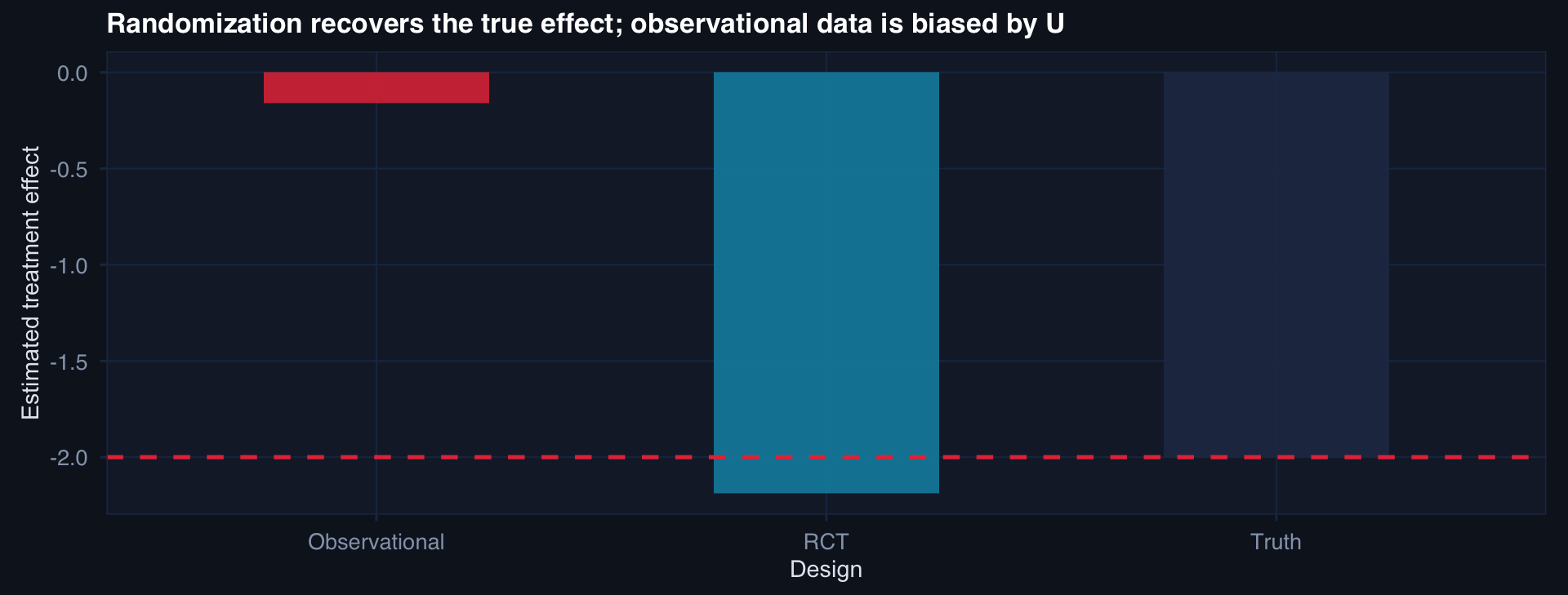
Randomization makes \(P(A=1 \mid U) = 0.5\) regardless of U. The groups become comparable on everything — measured and unmeasured — in expectation.

RCT Designs: Parallel vs. Crossover

Parallel-group (standard)

Each patient receives one treatment
Groups compared between patients
Simple, unambiguous causal target
Requires larger n

Best for:

Treatments with lasting effects
Surgical interventions
When carryover is a concern

Crossover

Each patient receives both treatments (sequenced)
Patient is their own control
Fewer patients needed
Washout period required

Best for:

Chronic stable conditions
Pharmacokinetic studies
When carryover can be designed away

Trauma caveat: Crossover is almost never appropriate — injuries are acute, interventions are not reversible, and conditions are not stable.

Simulating an RCT: Allocation and Estimation

n <- 300
df_rct <- tibble(
  id        = 1:n,
  treated   = rep(c(1,0), each=n/2)[sample(n)],   # 1:1 allocation
  baseline  = rnorm(n, 28, 10),                     # ISS at enrollment
  outcome   = 12 - 2.5*treated + 0.2*baseline + rnorm(n, 0, 3)
)

# Unadjusted estimate (valid because randomized)
fit_unadj <- lm(outcome ~ treated, data=df_rct)
# Covariate-adjusted (more precise, not more valid)
fit_adj   <- lm(outcome ~ treated + baseline, data=df_rct)

broom::tidy(fit_unadj, conf.int=TRUE) |>
  bind_rows(broom::tidy(fit_adj, conf.int=TRUE)) |>
  filter(term=="treated") |>
  mutate(Model = c("Unadjusted", "Adjusted for baseline ISS"),
         across(where(is.numeric), round, 3)) |>
  select(Model, estimate, std.error, conf.low, conf.high)

# A tibble: 2 × 5
  Model                     estimate std.error conf.low conf.high
  <chr>                        <dbl>     <dbl>    <dbl>     <dbl>
1 Unadjusted                   -1.85     0.425    -2.68     -1.01
2 Adjusted for baseline ISS    -2.31     0.343    -2.98     -1.63

In an RCT, adjustment is optional — it improves precision, not validity. In an observational study, adjustment is essential — and may still be insufficient.

Part 2

Observational Study Design

Structure and discipline when randomization is unavailable

The Observational Design Spectrum

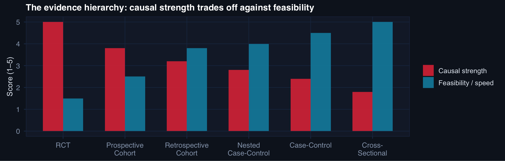
The best design is the one that can actually answer the question — within real-world constraints of time, cost, and ethics.

Cohort vs. Case-Control Logic

Cohort study

Start with exposure status
Follow forward → observe outcome
Estimates: RR, incidence rates, hazard ratios
Efficient when outcome is common
Prospective: best; retrospective: feasible

Exposed    →  Outcome?
Unexposed  →  Outcome?

Case-control study

Start with outcome status (cases vs. controls)
Look backward → exposure history
Estimates: OR (approximates RR when rare)
Efficient when outcome is rare
Control selection is the critical design decision

Cases    →  Were they exposed?
Controls →  Were they exposed?

DoDTR application: Studying rare complications (e.g., post-traumatic pulmonary embolism) → case-control. Studying treatment trajectories for all penetrating abdominal trauma → retrospective cohort.

The Bias That Design Controls

n <- 500
df_cohort <- tibble(
  exposed   = rbinom(n, 1, 0.45),
  confounder = rnorm(n),   # e.g., injury severity
  outcome   = rbinom(n, 1, plogis(-2 + 0.8*exposed + 1.2*confounder))
)

# Crude association
crude <- coef(glm(outcome ~ exposed, family=binomial, data=df_cohort))["exposed"]
# Adjusted
adj   <- coef(glm(outcome ~ exposed + confounder, family=binomial, data=df_cohort))["exposed"]

tibble(
  Estimator = c("Crude OR (exp)", "Adjusted OR (exp)", "True log-OR"),
  Value = round(c(exp(crude), exp(adj), exp(0.8)), 3)
)

# A tibble: 3 × 2
  Estimator         Value
  <chr>             <dbl>
1 Crude OR (exp)     2.52
2 Adjusted OR (exp)  3.09
3 True log-OR        2.23

Design controls selection bias (who enters the study). Analysis controls confounding (what else explains the association). Both must be addressed — design errors cannot be fixed in analysis.

Part 3

Cross-Sectional Design

Fast, practical — and easy to misinterpret

What a Cross-Sectional Study Can and Cannot Tell You

# Prevalence estimation from a cross-sectional survey
n <- 600
df_cs <- tibble(
  age_group = sample(c("18-30","31-45","46-60","60+"), n, replace=TRUE,
                     prob=c(0.3, 0.3, 0.25, 0.15)),
  site      = sample(c("Role 2","Role 3","Role 4"), n, replace=TRUE),
  cpg_compliant = rbinom(n, 1,
    ifelse(age_group=="18-30", 0.82,
    ifelse(age_group=="31-45", 0.76,
    ifelse(age_group=="46-60", 0.70, 0.65))))
)

df_cs |>
  group_by(age_group, site) |>
  summarise(prevalence = mean(cpg_compliant), n=n(), .groups="drop") |>
  ggplot(aes(age_group, prevalence, fill=site)) +
  geom_col(position="dodge", alpha=0.85) +
  geom_hline(yintercept=0.80, linetype=2, color="#e63946") +
  scale_fill_manual(values=c("#2563eb","#0891b2","#8b5cf6")) +
  scale_y_continuous(labels=scales::percent_format()) +
  labs(title="CPG compliance prevalence by age group and care level — cross-sectional snapshot",
       x="Age group", y="Compliance rate", fill="Care level") +
  theme_di()

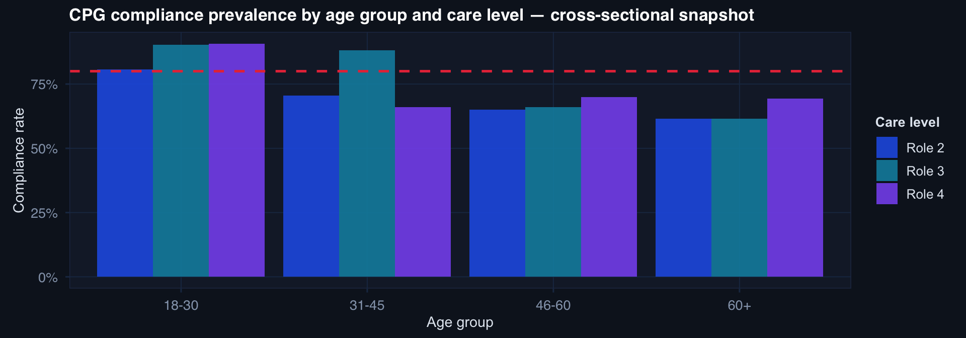
What this tells us: Prevalence at a point in time, stratified by observable characteristics.

What this cannot tell us: Whether compliance caused outcomes, or which direction the association runs.

Reverse Causation — The Cross-Sectional Trap

The temporality problem:

Cross-sectional studies measure exposure and outcome simultaneously. We cannot determine which came first.

Classic example: A cross-sectional survey finds that hospitalized patients have higher medication use. Does medication cause hospitalization — or does hospitalization cause more medications to be prescribed?

In registry analytics: A cross-sectional look at documentation completeness and patient severity may show high-severity patients have less complete records — but this reflects documentation capacity under pressure, not a causal relationship.

When cross-sectional is the right design:

Estimating prevalence of a condition
Screening and needs assessment
Baseline characterization before a longitudinal study
Rapid situational awareness (e.g., theater health surveys)
Hypothesis generation for causal studies

Lecture 1 — Key Takeaways

RCTs

Randomization breaks the confounder–treatment link
Parallel-group: standard; crossover: rare in acute settings
Covariate adjustment improves precision, not validity
Internal validity is highest — external validity requires thought

Observational Design

Cohort: starts with exposure, estimates RR
Case-control: starts with outcome, efficient for rare events
Confounding = design + analysis problem
Selection bias = design problem only

Cross-Sectional

Snapshot: estimates prevalence efficiently
Cannot establish temporality
Reverse causation is always a threat
Best for hypothesis generation, not causal confirmation

The meta-lesson: Design determines what questions can be answered. No amount of analytical sophistication converts a cross-sectional association into a causal estimate. Choose the design that matches the question.

Coming Up: Lecture 2

Longitudinal Design, Sample Size & Randomization Strategy

Posts 04, 05 & 06:

Longitudinal studies — trajectories, attrition, mixed-effects thinking
Sample size & power — effect sizes, simulation-based planning, sensitivity
Randomization & stratification — block randomization, minimization, balance diagnostics

Read Before Lecture 2