Inference — Estimating and Testing from Data

Applied Statistics for AI & Clinical Decision-Making — Lecture 3 of 10

Jonathan D. Stallings, PhD, MS

Data InDeed | dataindeed.org

2026-01-01

A p-value does not tell you what you think it tells you.

What You’ll Learn Today

Post 7 Beyond p < 0.05

• What a p-value actually is
• Type I & II errors
• Effect size > significance

Post 8 Confidence Intervals

• Correct interpretation
• Width, precision, n
• Why CIs beat p-values

Post 9 Maximum Likelihood

• The logic of MLE
• Score equations
• MLE unifies most models

Part 1

Beyond p < 0.05

Hypothesis testing in the age of AI

What a p-value Actually Is

p-value = P(observing data this extreme or more | H₀ is true)

What it is NOT:

• P(H₀ is true)
• P(you made a mistake)
• A measure of effect size
• A measure of clinical importance

null_df <- tibble::tibble(t = seq(-4, 4, 0.01), y = dt(t, df = 98))
obs_t <- 2.3
ggplot2::ggplot(null_df, aes(t, y)) +
  geom_line(linewidth = 1, color = "#475569") +
  geom_area(data = filter(null_df, t >= obs_t), fill = "#e63946", alpha = 0.7) +
  geom_area(data = filter(null_df, t <= -obs_t), fill = "#e63946", alpha = 0.7) +
  geom_vline(xintercept = c(-obs_t, obs_t), linetype = 2) +
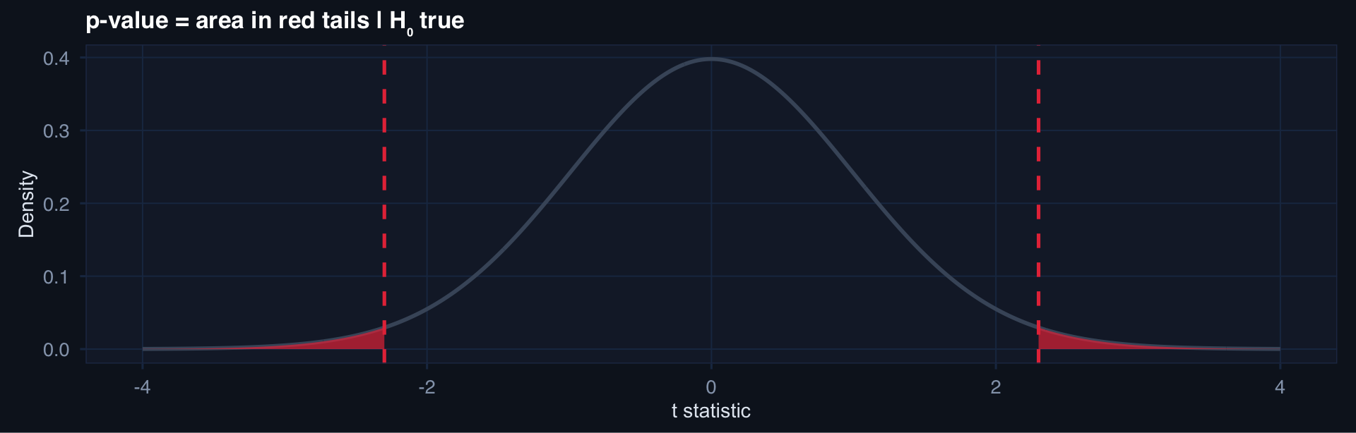
  labs(title = "p-value = area in red tails | H₀ true", x = "t statistic", y = "Density") + theme_di()

This is the most misunderstood concept in statistics. The p-value is a conditional probability under a hypothesis we often know is false. It is NOT the probability the null is true, and it says nothing about clinical importance.

Type I and Type II Errors

	H₀ True	H₀ False
Reject H₀	Type I error (α)	✅ Correct (Power = 1-β)
Fail to reject	✅ Correct	Type II error (β)

In clinical AI the asymmetry matters:

Trauma triage model:

• Type I error = flag patient who doesn’t need intervention → wasted resources
• Type II error = miss patient who does need intervention → preventable death

The cost of these errors is not symmetric. Setting α = 0.05 arbitrarily ignores this.

In academic statistics, Type I error is treated as the primary concern by convention. In clinical settings, Type II errors (missed cases) are often far more costly. The choice of significance threshold should reflect the relative cost of each error type — not convention.

Effect Size: What Significance Ignores

Statistical significance ≠ clinical significance

set.seed(42)
n_large <- 5000; n_small <- 50
df_large <- tibble(group = rep(c("A","B"), each=n_large),
                   y = c(rnorm(n_large,0,1), rnorm(n_large,0.05,1)))
df_small <- tibble(group = rep(c("A","B"), each=n_small),
                   y = c(rnorm(n_small,0,1), rnorm(n_small,0.8,1)))

p_large <- t.test(y~group, data=df_large)$p.value
p_small <- t.test(y~group, data=df_small)$p.value

tibble::tibble(
  Dataset = c("n=5000/group, d=0.05", "n=50/group, d=0.80"),
  `p-value` = round(c(p_large, p_small), 4),
  `Effect size (d)` = c(0.05, 0.80),
  `Clinical importance` = c("Negligible", "Large")
)

# A tibble: 2 × 4
  Dataset              `p-value` `Effect size (d)` `Clinical importance`
  <chr>                    <dbl>             <dbl> <chr>                
1 n=5000/group, d=0.05    0.0053              0.05 Negligible           
2 n=50/group, d=0.80      0                   0.8  Large                

Lesson: Large n detects trivially small effects. Small n misses large ones.

This is the practical lesson from hypothesis testing that most courses bury in a footnote. With 5000 patients per group you can achieve p < 0.05 for a difference of 0.05 standard deviations — a difference with no clinical meaning. Report effect sizes alongside p-values, always.

Part 2

Confidence Intervals

The honest way to report estimation uncertainty

What a Confidence Interval Actually Means

A 95% CI means: if we repeated this study 100 times, approximately 95 of the resulting intervals would contain the true parameter.

It does NOT mean: “there is a 95% probability the true value is in this interval”

simulate_ci <- function(id) {
  x <- rnorm(40, mean=0.30, sd=0.10)
  ci <- t.test(x)$conf.int
  tibble(id=id, lower=ci[1], upper=ci[2], contains_true = ci[1] <= 0.30 & ci[2] >= 0.30)
}
ci_df <- purrr::map_dfr(1:50, simulate_ci)
ggplot2::ggplot(ci_df, aes(x=id, ymin=lower, ymax=upper, color=contains_true)) +
  geom_errorbar(linewidth=0.6) +
  geom_hline(yintercept=0.30, linetype=2, color="#e63946") +
  scale_color_manual(values=c("FALSE"="#e63946","TRUE"="#2563eb")) +
  coord_flip() + theme_di() +
  labs(title="50 simulated 95% CIs — ~5% miss the true value (red)",
       x="Simulation", y="Interval", color="Contains true value")

The correct frequentist interpretation of a CI is about procedure, not probability. The interval from this specific study either contains the true value or it doesn’t. We just don’t know which. The 95% refers to the long-run coverage of the procedure. That said, in practice, treating a 95% CI as “the plausible range” is a useful approximation.

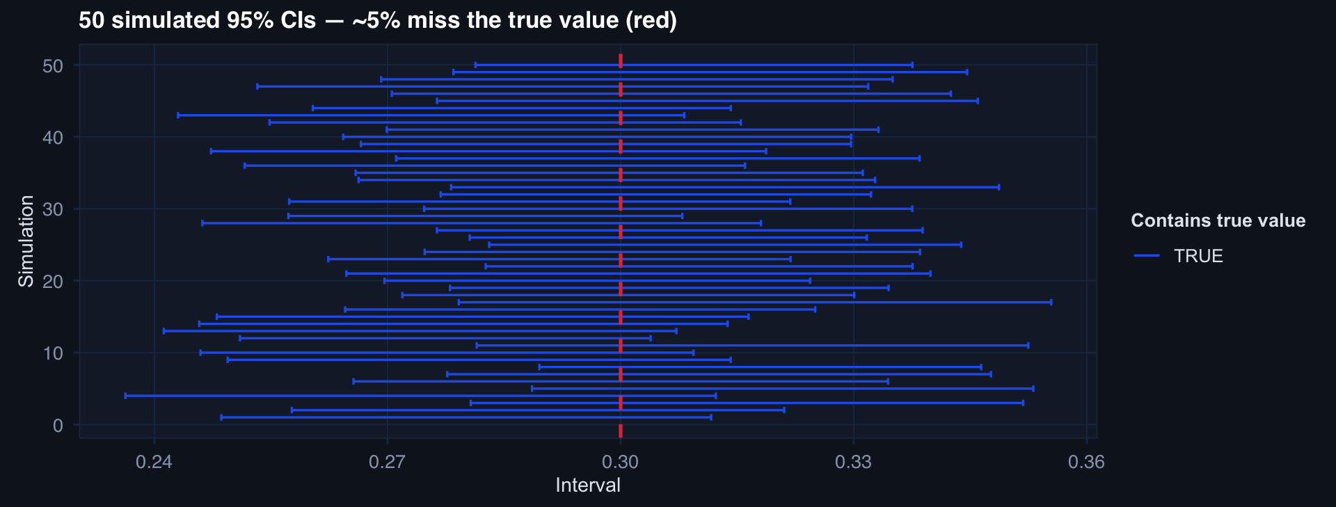
CI Width Tells You About Precision

ci_widths <- tibble::tibble(
  n = c(20, 50, 100, 200, 500, 1000),
  width = 2 * qt(0.975, df = n-1) * (0.15 / sqrt(n))
)
ggplot2::ggplot(ci_widths, aes(x=n, y=width)) +
  geom_line(linewidth=1.2, color="#2563eb") +
  geom_point(size=3, color="#1b2e4b") +
  labs(title="95% CI width vs. sample size (σ = 0.15)",
       x="n", y="CI width (percentage points)") + theme_di()

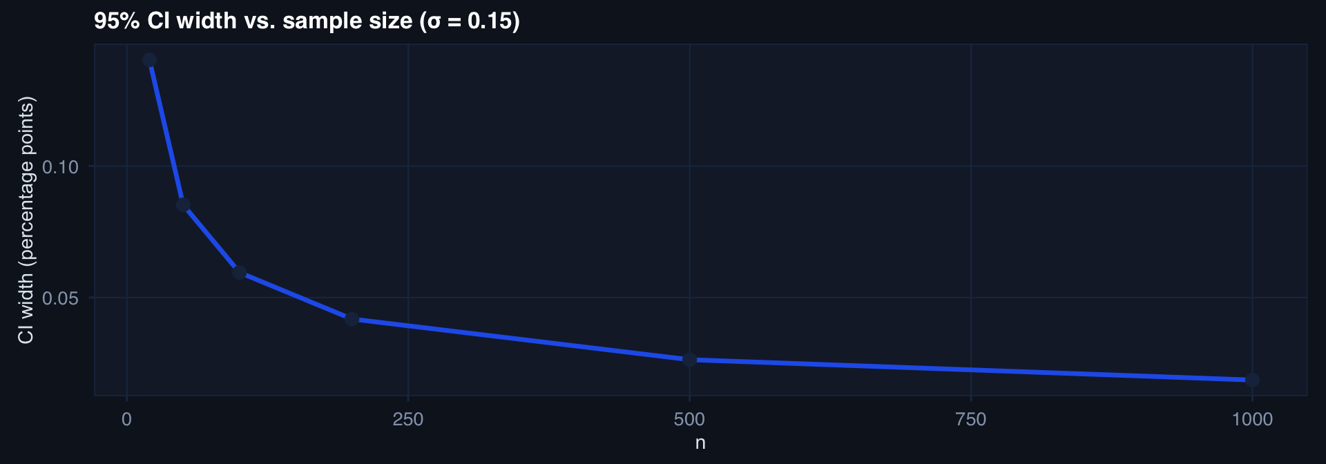
Registry reporting: A 95% CI of [0.23, 0.41] for a CPG compliance rate tells commanders the range of plausible true compliance — far more actionable than “p = 0.003.”

Part 3

Maximum Likelihood Estimation

The unifying framework behind most models

The Intuition Behind MLE

Find the parameter values that make the observed data most probable.

\[\hat{\theta}_{MLE} = \arg\max_\theta \; \mathcal{L}(\theta \mid \text{data}) = \arg\max_\theta \prod_{i=1}^n f(x_i \mid \theta)\]

In practice: maximize the log-likelihood \(\ell(\theta) = \sum_i \log f(x_i \mid \theta)\)

Why it matters:

• Logistic regression → maximizes Bernoulli log-likelihood
• Linear regression → MLE = OLS when errors are Normal
• Poisson regression → maximizes Poisson log-likelihood
• Survival models → maximizes partial likelihood

MLE is the engine underneath almost every model in this series.

MLE unifies a huge range of seemingly different methods. Once students understand that fitting a logistic regression IS maximizing a log-likelihood, and that the coefficients are the parameter values that maximize P(observed outcomes | predictors, β), the entire family of GLMs becomes conceptually unified.

MLE in Action: Fitting a Bernoulli Model

# Trauma mortality: find MLE of p from n=50 patients, 12 deaths
n_patients <- 50; n_deaths <- 12

# Log-likelihood surface
p_grid <- seq(0.01, 0.99, 0.001)
log_lik <- dbinom(n_deaths, size=n_patients, prob=p_grid, log=TRUE)

mle_p <- p_grid[which.max(log_lik)]

tibble::tibble(p = p_grid, log_lik = log_lik) |>
  ggplot2::ggplot(aes(p, log_lik)) +
  geom_line(linewidth=1.2, color="#2563eb") +
  geom_vline(xintercept=mle_p, linetype=2, color="#e63946") +
  annotate("text", x=mle_p+0.06, y=-25,
           label=paste0("MLE = ", mle_p), color="#e63946") +
  labs(title="Log-likelihood for mortality rate p",
       x="p (mortality rate)", y="Log-likelihood") + theme_di()

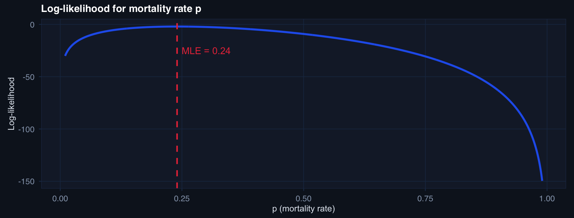
MLE = 12/50 = 0.24 — exactly the sample proportion. The math confirms the intuition.

Lecture 3 — Key Takeaways

Hypothesis Testing

• p-value = P(data | H₀) — not P(H₀ | data)
• Type I/II error tradeoffs are asymmetric in clinical settings
• Effect size always alongside p-value
• Significance thresholds should reflect error costs

Confidence Intervals

• Frequentist procedure — not a probability statement about one interval
• Width = precision = function of n and σ
• Report CIs instead of (or alongside) p-values

MLE

• Find θ that maximizes P(observed data | θ)
• Maximize log-likelihood in practice
• Unifies linear, logistic, Poisson, survival models
• OLS = MLE when residuals are Normal

The meta-lesson: Inference is about characterizing uncertainty honestly — not just getting below 0.05.

Coming Up: Lecture 4

Bayesian Methods & Simulation

The frequentist framework asks: what is P(data | parameter)? The Bayesian framework asks: what is P(parameter | data)?

Posts 10, 27, 23:

• Bayesian Thinking — priors, likelihoods, posteriors
• Monte Carlo — simulating when math is intractable
• Entropy — information, uncertainty, KL divergence

Read Before Lecture 4

• Bayesian Thinking
• Monte Carlo Magic
• Entropy in Stats