Bayesian Methods & Simulation

Applied Statistics for AI & Clinical Decision-Making — Lecture 4 of 10

Jonathan D. Stallings, PhD, MS

Data InDeed | dataindeed.org

2026-01-01

Bayesian inference is not a philosophy. It is a computational framework.

What You’ll Learn Today

Post 10 Bayesian Thinking

• Priors, likelihoods, posteriors
• Conjugate updates
• Posterior predictive distributions

Post 27 Monte Carlo Methods

• Monte Carlo integration
• Importance sampling
• MCMC & Metropolis-Hastings

Post 23 Entropy & Information

• Shannon entropy
• KL divergence
• Information in model selection

Part 1

Bayesian Thinking

Updating belief with evidence

The Bayesian Framework

\[\underbrace{P(\theta \mid y)}_{\text{posterior}} \propto \underbrace{P(y \mid \theta)}_{\text{likelihood}} \times \underbrace{P(\theta)}_{\text{prior}}\]

Three components:

• Prior \(P(\theta)\) — what you believe before seeing data
• Likelihood \(P(y|\theta)\) — how probable is the data given the parameter
• Posterior \(P(\theta|y)\) — updated belief after seeing data

The Bayesian advantage in small samples:

When registry data is sparse (rare injury, small cohort), a sensible prior prevents the model from overfitting to noise.

CPG compliance example:

Prior: historical compliance ~70% based on previous quarter.

New data: 14/20 cases compliant this quarter.

Posterior: updated estimate that appropriately shrinks toward the prior when n is small.

The frequentist approach says: the parameter is fixed, we compute P(data | parameter). The Bayesian approach says: we have uncertainty about the parameter, we compute P(parameter | data). For clinical problems with small samples, strong prior knowledge, and the need to communicate uncertainty directly, Bayesian methods are often more appropriate.

Conjugate Updating: Beta-Binomial

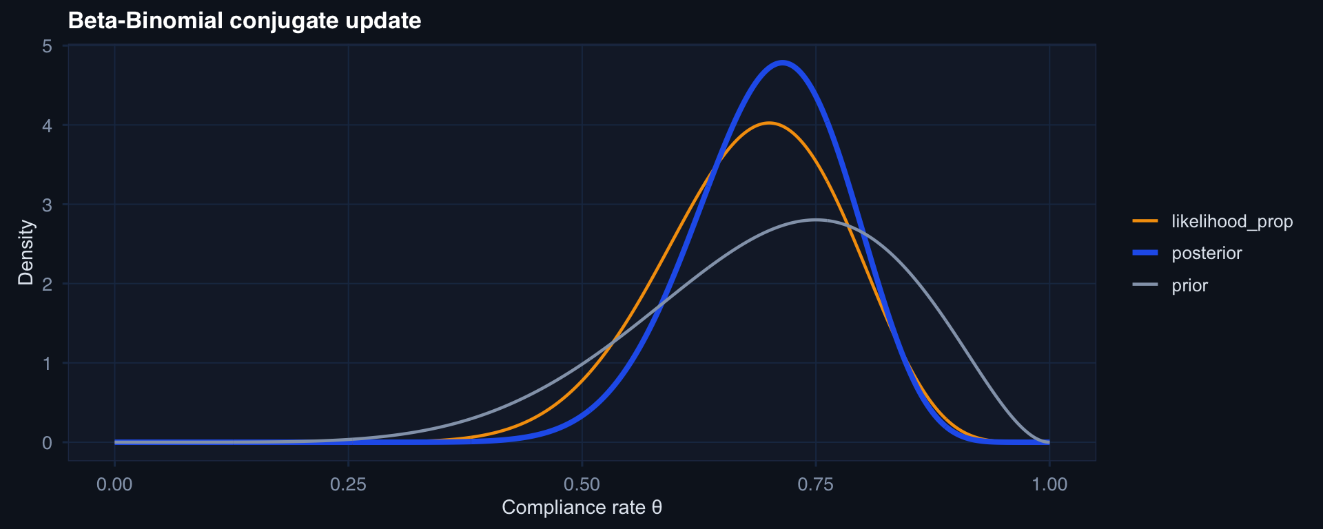
# Prior: Beta(7, 3) → prior belief ~70% compliance
# Data: 14/20 compliant
# Posterior: Beta(7+14, 3+6) = Beta(21, 9)

theta <- seq(0, 1, 0.001)
prior     <- dbeta(theta, 7, 3)
likelihood_prop <- dbeta(theta, 15, 7)   # normalized for display
posterior <- dbeta(theta, 21, 9)

tibble(theta, prior, likelihood_prop, posterior) |>
  tidyr::pivot_longer(-theta) |>
  ggplot(aes(theta, value, color=name, linewidth=name)) +
  geom_line() +
  scale_color_manual(values=c("prior"="#94a3b8","likelihood_prop"="#f59e0b","posterior"="#2563eb")) +
  scale_linewidth_manual(values=c("prior"=0.8,"likelihood_prop"=0.8,"posterior"=1.4)) +
  labs(title="Beta-Binomial conjugate update",
       x="Compliance rate θ", y="Density", color=NULL, linewidth=NULL) + theme_di()

This is the cleanest demonstration of Bayesian updating. The prior (gray) encodes our historical knowledge. The likelihood (yellow) encodes what this quarter’s data tells us. The posterior (blue) is the combination — it’s pulled toward the prior when the data is sparse, and toward the likelihood when the data is abundant. The posterior mean is (21)/(21+9) = 0.70 — the data and prior agree here, so the posterior is confident.

Posterior Predictive Distribution

# Posterior Beta(21,9) — predict next 20 patients
n_sims <- 10000; n_next <- 20
theta_sims <- rbeta(n_sims, 21, 9)
y_pred     <- rbinom(n_sims, n_next, theta_sims)

tibble(compliant = y_pred) |>
  ggplot(aes(x=compliant)) +
  geom_bar(fill="#2563eb", alpha=0.8) +
  geom_vline(xintercept=mean(y_pred), linetype=2, color="#e63946") +
  labs(title="Posterior predictive: compliant cases in next 20 patients",
       x="# compliant", y="Count") + theme_di()

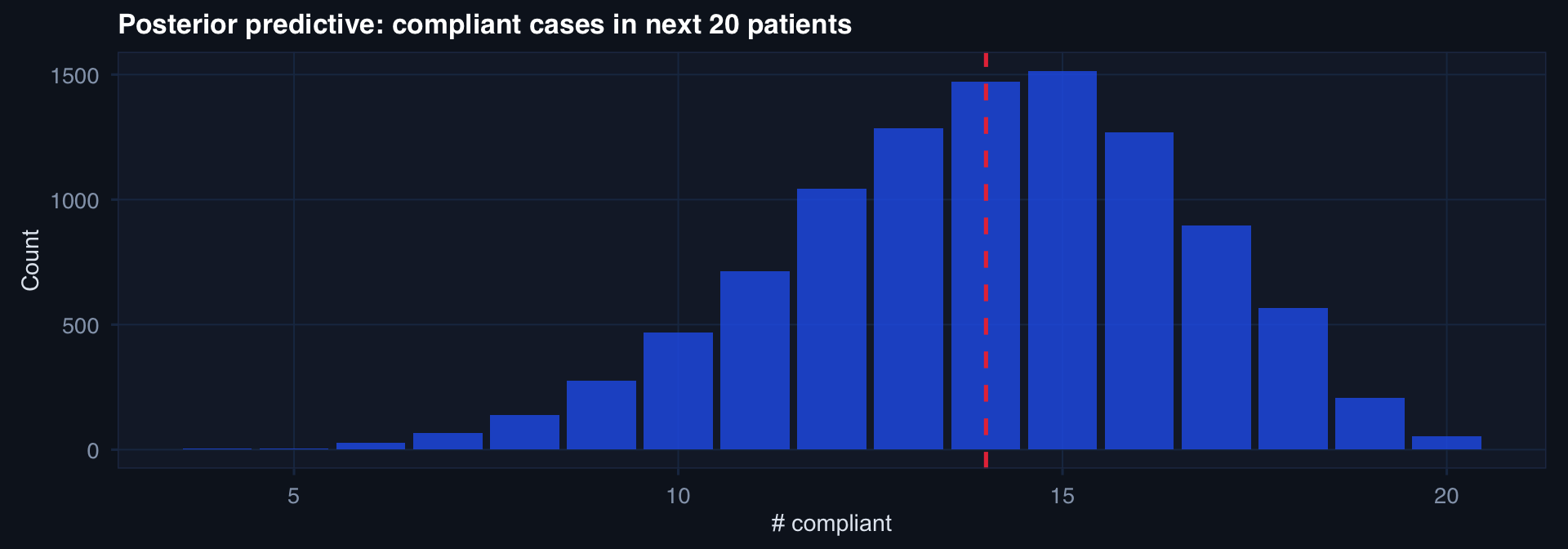
The posterior predictive propagates parameter uncertainty into outcome uncertainty — the right thing to give commanders.

Part 2

Monte Carlo Methods

When the math is intractable, simulate

The Core Monte Carlo Idea

\[E_p[g(X)] \approx \frac{1}{n}\sum_{i=1}^n g(X_i), \quad X_i \sim p(x)\]

Simulate → transform → average.

# Classic: estimate π by random points in unit square
n <- 10000
pts <- tibble(x=runif(n), y=runif(n)) |>
  mutate(inside = (x^2 + y^2) <= 1)

pi_est <- 4 * mean(pts$inside)
cat("Monte Carlo π estimate:", round(pi_est, 4), "\n")

Monte Carlo π estimate: 3.1264 

ggplot(pts[1:2000,], aes(x, y, color=inside)) +
  geom_point(size=0.4, alpha=0.6) +
  scale_color_manual(values=c("FALSE"="#e63946","TRUE"="#2563eb")) +
  coord_fixed() + theme_di() +
  labs(title=paste0("Estimating π via Monte Carlo (n=2000 shown) ≈ ", round(pi_est,3)))

The π estimation example is pedagogically important because the true answer is known. Students can see that Monte Carlo gets close but isn’t exact — and that more simulations gets closer. This directly applies to posterior integrals that have no closed form.

MCMC: Sampling from Intractable Posteriors

When we can’t sample directly, build a Markov chain that converges to the target.

# Metropolis-Hastings targeting N(0,1)
n_iter <- 4000; chain <- numeric(n_iter); chain[1] <- 5
for(i in 2:n_iter) {
  prop <- rnorm(1, chain[i-1], 0.8)
  log_a <- dnorm(prop,log=TRUE) - dnorm(chain[i-1],log=TRUE)
  chain[i] <- if(log(runif(1)) < log_a) prop else chain[i-1]
}

tibble(iter=1:n_iter, value=chain) |>
  ggplot(aes(iter, value)) +
  geom_line(linewidth=0.35, color="#2563eb") +
  geom_hline(yintercept=0, linetype=2, color="#e63946") +
  labs(title="Metropolis-Hastings trace plot — targeting N(0,1)",
       x="Iteration", y="Sample") + theme_di()

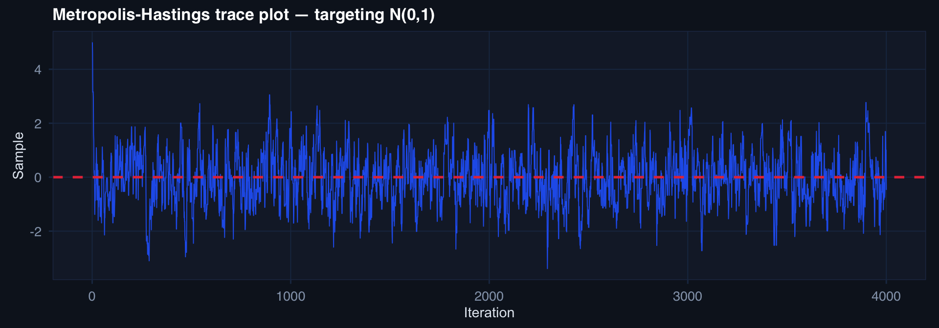
Bayesian trauma model: MCMC lets us fit hierarchical models with random effects for facility, time period, and injury pattern — posteriors that have no closed form but can be sampled.

Part 3

Entropy & Information Theory

Quantifying uncertainty in data and models

Shannon Entropy: Measuring Uncertainty

\[H(X) = -\sum_{x} P(x) \log_2 P(x)\]

Units: bits (base 2) or nats (base e)

entropy <- function(p) -sum(p[p>0] * log2(p[p>0]))
probs <- seq(0.01, 0.99, 0.01)
entropies <- sapply(probs, function(p) entropy(c(p, 1-p)))

tibble(p=probs, H=entropies) |>
  ggplot(aes(p, H)) +
  geom_line(linewidth=1.3, color="#2563eb") +
  geom_vline(xintercept=0.5, linetype=2, color="#e63946") +
  labs(title="Entropy of a binary outcome — max at p=0.5",
       x="P(event)", y="Entropy H (bits)") + theme_di()

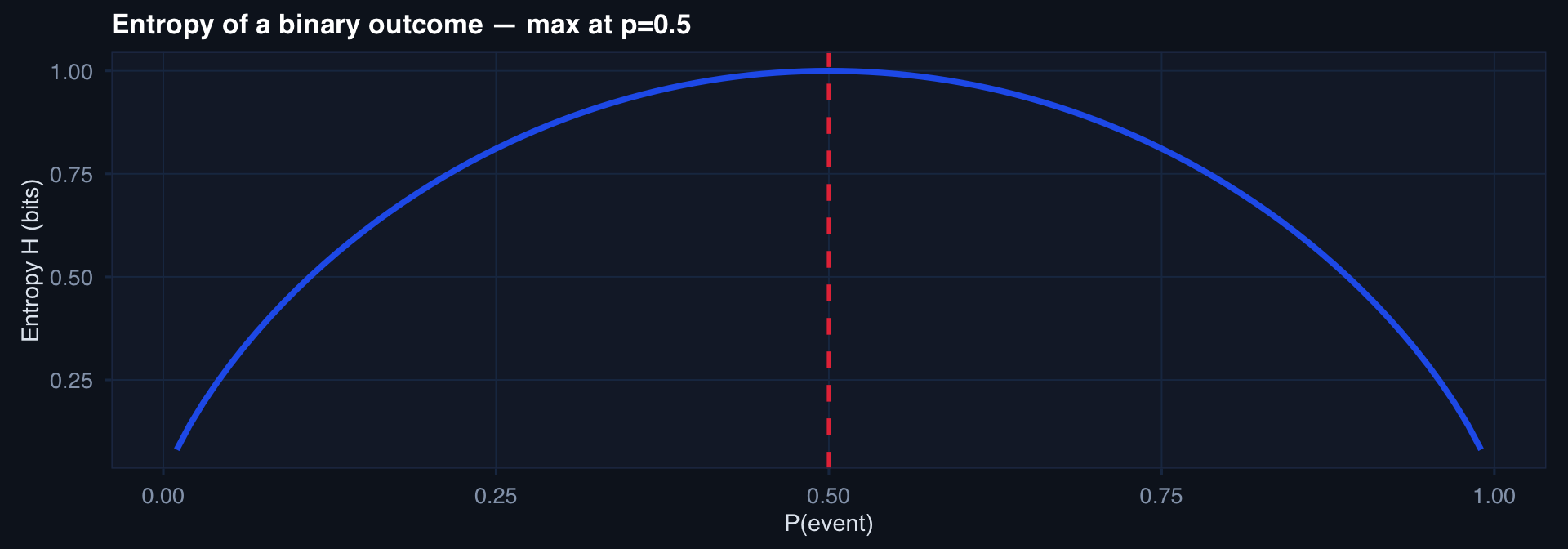
High entropy = high uncertainty (50/50 coin flip). Low entropy = low uncertainty (rare event we’re nearly certain about).

KL Divergence & Model Selection

\[D_{KL}(P \| Q) = \sum_x P(x) \log \frac{P(x)}{Q(x)} \geq 0\]

Interpretation: How much information is lost when Q is used to approximate P.

Applications in clinical AI:

• Cross-entropy loss in neural networks = KL divergence from true labels
• AIC/BIC penalize models with more parameters (information-theoretic basis)
• WAIC (widely applicable information criterion) — Bayesian model comparison

Model selection for trauma outcomes: When comparing a logistic model vs. a flexible ML model for mortality, AIC/BIC/WAIC all operationalize the same idea: penalize complexity, reward fit. KL divergence is the underlying concept.

Lecture 4 — Key Takeaways

Bayesian Methods

• Posterior ∝ Likelihood × Prior
• Conjugate priors allow closed-form updating
• Posterior predictive propagates uncertainty forward
• Ideal for small-n clinical problems with prior knowledge

Monte Carlo

• Simulate → transform → average
• MCMC samples from intractable posteriors
• Trace plots and R̂ diagnose convergence
• Powers Bayesian modeling in practice

Entropy

• H(X) measures average surprise/uncertainty
• Maximum entropy = uniform distribution
• KL divergence = information lost using wrong model
• Foundation of cross-entropy loss, AIC, model selection

The meta-lesson: Bayesian + simulation methods together handle any posterior, regardless of analytic tractability.

Coming Up: Lecture 5

Regression — The Workhorse Models

“All models are wrong, but some are useful.” — Box

Posts 11, 12, 13:

• Linear Regression — OLS, assumptions, diagnostics
• Logistic Regression — binary outcomes, odds ratios, calibration
• GLMs — the unified family connecting all regression models

Read Before Lecture 5

• Linear Regression Still Matters
• Logistic Regression: Predicting Yes/No
• GLMs: Flexible Modeling