Regression — The Workhorse Models

Applied Statistics for AI & Clinical Decision-Making — Lecture 5 of 10

Jonathan D. Stallings, PhD, MS

Data InDeed | dataindeed.org

2026-01-01

Regression models the conditional mean. Everything else is a generalization of that idea.

What You’ll Learn Today

Post 11 Linear Regression

• OLS geometry
• Assumptions & diagnostics
• Prediction vs. inference

Post 12 Logistic Regression

• Binary outcomes
• Log-odds and odds ratios
• Calibration matters

Post 13 GLMs

• The exponential family
• Link functions
• Poisson, Gamma, NB

Part 1

Linear Regression

Still the most important model in statistics

OLS: The Normal Equations

\[\hat{\beta} = (X^\top X)^{-1} X^\top y\]

Minimize: \(\text{RSS} = \sum_{i=1}^n (y_i - \hat{y}_i)^2\)

n <- 200
df <- tibble(
  iss = rnorm(n, 25, 12),
  los = 2 + 0.4 * iss + rnorm(n, 0, 5)
)
fit <- lm(los ~ iss, data = df)
df$fitted <- fitted(fit)

ggplot(df, aes(iss, los)) +
  geom_point(alpha=0.4, color="#475569") +
  geom_smooth(method="lm", color="#2563eb", se=TRUE) +
  labs(title="Linear regression: ISS → Hospital LOS",
       x="Injury Severity Score", y="Length of Stay (days)") + theme_di()

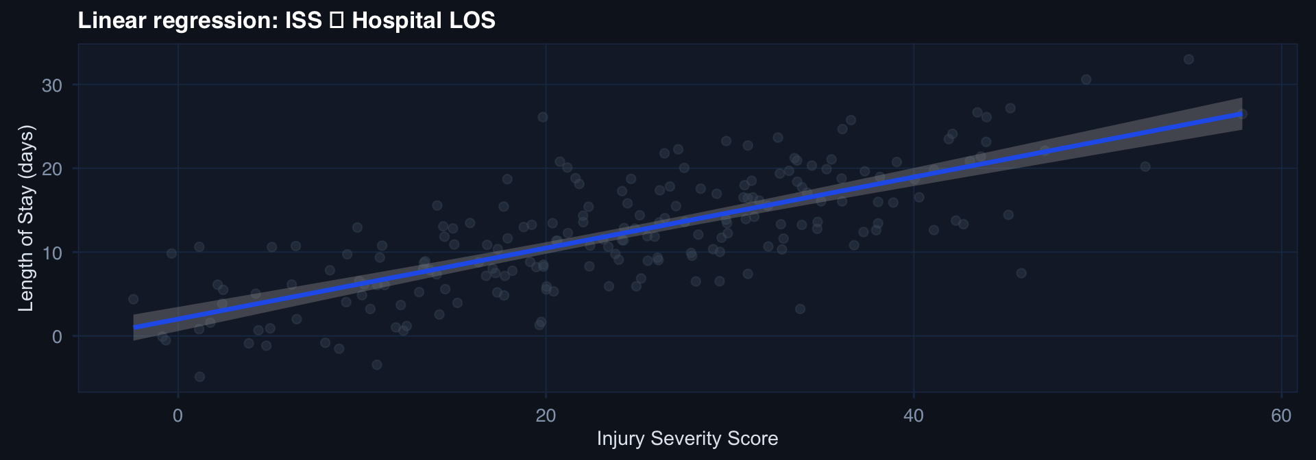
Coefficient interpretation: β = 0.40 means each 1-point increase in ISS is associated with 0.4 additional days of LOS, holding all other predictors constant.

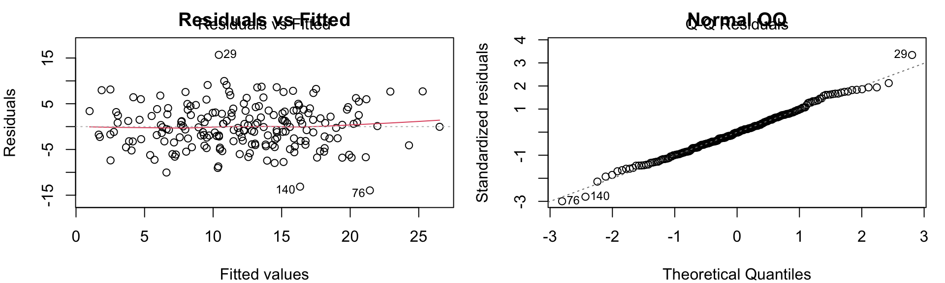
The Four OLS Assumptions (L-I-N-E)

Assumption	What it means	How to check
Linearity	E[Y|X] is linear in X	Residual vs. fitted plot
Independence	Observations independent	Study design, ACF plot
Normality	Residuals ~ Normal	QQ plot
Equal variance	Var(ε) constant	Scale-location plot

par(mfrow=c(1,2), mar=c(4,4,2,1))
plot(fit, which=1, main="Residuals vs Fitted")
plot(fit, which=2, main="Normal QQ")

In trauma registry work, independence is often the most violated assumption — patients at the same facility share features that make their outcomes correlated. This is why mixed models and clustered standard errors matter in registry analyses.

Part 2

Logistic Regression

The gold standard for binary clinical outcomes

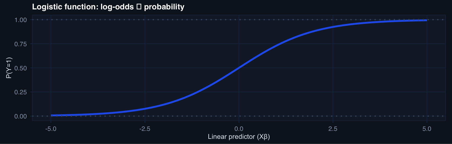
Why Not Linear Regression for Binary Outcomes?

Linear regression on a 0/1 outcome produces predicted probabilities outside [0,1].

The logistic solution: model the log-odds.

\[\log\frac{P(Y=1)}{P(Y=0)} = \beta_0 + \beta_1 X_1 + \dots\]

\[P(Y=1) = \frac{e^{X\beta}}{1 + e^{X\beta}} = \text{logistic}(X\beta)\]

x <- seq(-5,5,0.05)
tibble(x=x, prob=plogis(x)) |>
  ggplot(aes(x,prob)) +
  geom_line(linewidth=1.4, color="#2563eb") +
  geom_hline(yintercept=c(0,1), linetype=3, color="#475569") +
  labs(title="Logistic function: log-odds → probability",
       x="Linear predictor (Xβ)", y="P(Y=1)") + theme_di()

Fitting and Interpreting Logistic Regression

n <- 500
df_log <- tibble(
  sbp    = rnorm(n, 110, 20),
  iss    = rnorm(n, 28, 14),
  died   = rbinom(n, 1, plogis(-3 + 0.02*iss - 0.01*sbp))
)
fit_log <- glm(died ~ iss + sbp, family=binomial, data=df_log)
broom::tidy(fit_log, exponentiate=TRUE, conf.int=TRUE) |>
  dplyr::select(term, estimate, conf.low, conf.high, p.value) |>
  dplyr::rename(OR=estimate) |>
  dplyr::mutate(across(where(is.numeric), ~round(.,3)))

# A tibble: 3 × 5
  term           OR conf.low conf.high p.value
  <chr>       <dbl>    <dbl>     <dbl>   <dbl>
1 (Intercept) 0.051    0.003     0.747   0.035
2 iss         1.03     0.999     1.06    0.06 
3 sbp         0.988    0.965     1.01    0.324

Odds ratio interpretation: OR = 1.02 for ISS means each 1-unit increase in ISS multiplies the odds of death by 1.02 (2% increase per ISS point).

Logistic regression is the foundation of clinical prediction models. It’s what TRISS, APACHE, and most trauma mortality models are built on. Understanding its mechanics — log-odds, odds ratios, the logistic link — is essential before moving to more complex models.

Calibration: The Most Important Model Property

df_log$pred_prob <- predict(fit_log, type="response")
df_log |>
  dplyr::mutate(decile = ntile(pred_prob, 10)) |>
  dplyr::group_by(decile) |>
  dplyr::summarise(mean_pred=mean(pred_prob), obs_rate=mean(died)) |>
  ggplot(aes(mean_pred, obs_rate)) +
  geom_abline(linetype=2, color="#94a3b8") +
  geom_point(size=3, color="#2563eb") +
  geom_line(color="#2563eb") +
  labs(title="Calibration plot: predicted vs. observed mortality",
       x="Mean predicted probability", y="Observed rate") + theme_di()

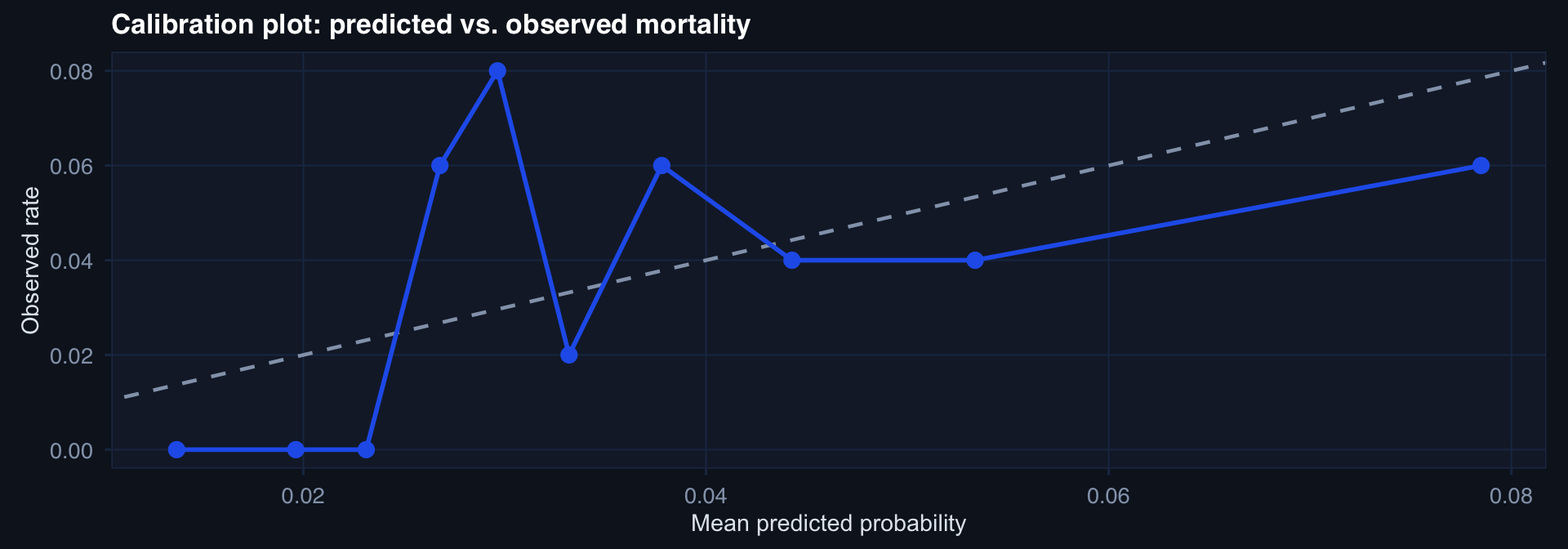
A model that says “30% mortality risk” should be wrong about 70% of the time. Calibration measures whether the model’s confidence matches reality. A discriminating but miscalibrated model gives overconfident wrong answers — dangerous in clinical triage.

Part 3

Generalized Linear Models

One framework, unlimited distributions

The GLM Unification

\[g(E[Y]) = X\beta\]

Link function \(g(\cdot)\) connects the mean to the linear predictor.

Distribution	Link	Use case
Normal	identity	Continuous outcomes (LOS, scores)
Binomial	logit	Binary outcomes (mortality, complication)
Poisson	log	Count outcomes (readmissions, procedures)
Gamma	log or inverse	Right-skewed positive continuous (cost)
Negative Binomial	log	Overdispersed counts

# Count model: transfusions ~ ISS
df_count <- tibble(iss=rnorm(300,28,12), units=rpois(300, exp(0.5 + 0.03*iss)))
fit_pois <- glm(units ~ iss, family=poisson, data=df_count)
exp(coef(fit_pois))  # Rate ratios

(Intercept)         iss 
   1.512177    1.031848 

Lecture 5 — Key Takeaways

Linear Regression

• OLS minimizes RSS → normal equations
• Check L-I-N-E assumptions
• Violations → clustered SEs, mixed models
• Prediction vs. inference use different diagnostics

Logistic Regression

• Models log-odds of binary outcome
• Coefficients → odds ratios via exp()
• Always plot calibration, not just AUC
• MLE under Bernoulli likelihood

GLMs

• One framework: exponential family + link function
• Poisson → count data
• Gamma/log-Normal → right-skewed continuous
• Model selection: AIC, likelihood ratio tests

The meta-lesson: Linear, logistic, and GLMs are the same model with different distributional assumptions. Master the framework, not just the special cases.

Coming Up: Lecture 6

Comparing Groups & Special Methods

Posts 14, 18, 19:

• ANOVA — extending regression to multiple groups
• Survival Analysis — time-to-event with censoring
• Non-Parametric — when distributional assumptions fail

Read Before Lecture 6

• ANOVA in ML
• Survival Analysis
• Going Non-Parametric