Comparing Groups & Special Clinical Methods

Applied Statistics for AI & Clinical Decision-Making — Lecture 6 of 10

Jonathan D. Stallings, PhD, MS

Data InDeed | dataindeed.org

2026-01-01

Not all outcomes are continuous. Not all follow-up is complete. Not all distributions are Normal.

What You’ll Learn Today

Post 14 ANOVA

• One-way and two-way
• F-statistic logic
• Multiple comparisons

Post 18 Survival Analysis

• Time-to-event + censoring
• Kaplan-Meier curves
• Cox proportional hazards

Post 19 Non-Parametric

• Rank-based tests
• Wilcoxon, Kruskal-Wallis
• When to use them

Part 1

ANOVA

Regression in disguise — with more than two groups

ANOVA Is Just Regression

\[F = \frac{\text{Between-group variance (MS}_\text{between}\text{)}}{\text{Within-group variance (MS}_\text{within}\text{)}}\]

Large F → groups differ more than chance explains.

df_anova <- tibble(
  role = rep(c("Role 2","Role 3","Role 4"), each=80),
  iss  = c(rnorm(80,22,8), rnorm(80,30,10), rnorm(80,38,12))
)
fit_aov <- aov(iss ~ role, data=df_anova)
summary(fit_aov)

             Df Sum Sq Mean Sq F value   Pr(>F)    
role          2   8613    4306   38.45 3.46e-15 ***
Residuals   237  26544     112                     
---
Signif. codes:  0 '***' 0.001 '**' 0.01 '*' 0.05 '.' 0.1 ' ' 1

Registry application: Is mean ISS significantly different across Role 2, 3, and 4 care settings? ANOVA tests this without running three separate t-tests (which would inflate Type I error).

Multiple Comparisons: The Problem

# Bonferroni-corrected pairwise comparisons
pairwise.t.test(df_anova$iss, df_anova$role,
                p.adjust.method = "bonferroni")

    Pairwise comparisons using t tests with pooled SD 

data:  df_anova$iss and df_anova$role 

       Role 2  Role 3
Role 3 1.3e-05 -     
Role 4 1.1e-15 2e-04 

P value adjustment method: bonferroni 

Why correction matters: With 3 groups = 3 comparisons. Each at α=0.05 → ~14% chance of at least one false positive by chance alone. Bonferroni multiplies p-values by the number of comparisons.

Other options: Tukey HSD (preferred for ANOVA follow-up), Holm, Benjamini-Hochberg.

The multiple comparison problem is pervasive in clinical research. Every time you run an analysis on a registry with 68 CPG outcomes, you’re doing 68 simultaneous tests. Without correction, roughly 3-4 of those “significant” findings are false positives just by chance.

Part 2

Survival Analysis

When time matters and not everyone reaches the outcome

The Censoring Problem

Why ordinary regression fails for time-to-event data:

Patient A: died at day 45        → complete observation
Patient B: still alive at day 90 → right-censored (we know survival > 90 days)
Patient C: lost to follow-up day 30 → right-censored

Ignoring censored patients biases results toward shorter survival times.

Survival function: \(S(t) = P(T > t)\)

Hazard function: \(h(t) = \lim_{\Delta t \to 0} \frac{P(t \leq T < t+\Delta t \mid T \geq t)}{\Delta t}\)

The censoring concept is crucial and often misunderstood. A censored observation is not a missing outcome — it’s partial information. We know the patient survived at least to the censoring time. Ignoring them throws away real information and creates bias.

Kaplan-Meier Curves

df_surv <- tibble(
  time   = c(rexp(100, 0.02), rexp(100, 0.035)),
  status = rbinom(200, 1, 0.75),
  group  = rep(c("Standard","Damage Control"), each=100)
)
km_fit <- survfit(Surv(time, status) ~ group, data=df_surv)
plot(km_fit, col=c("#2563eb","#e63946"), lwd=2,
     xlab="Days", ylab="Survival probability",
     main="Kaplan-Meier: Standard vs. Damage Control Resuscitation")
legend("topright", levels(factor(df_surv$group)),
       col=c("#2563eb","#e63946"), lwd=2)

The KM curve is the first thing to plot for any time-to-event analysis. The step function drops every time an event occurs. The tick marks show censored observations. The log-rank test compares the curves formally.

Cox Proportional Hazards Model

\[h(t \mid X) = h_0(t) \cdot e^{\beta_1 X_1 + \beta_2 X_2 + \dots}\]

Hazard ratio = \(e^\beta\) — proportional change in hazard per unit increase in X.

fit_cox <- coxph(Surv(time, status) ~ group + rnorm(200), data=df_surv)
broom::tidy(fit_cox, exponentiate=TRUE, conf.int=TRUE) |>
  dplyr::mutate(across(where(is.numeric), ~round(.,3))) |>
  dplyr::select(term, estimate, conf.low, conf.high, p.value)

# A tibble: 2 × 5
  term          estimate conf.low conf.high p.value
  <chr>            <dbl>    <dbl>     <dbl>   <dbl>
1 groupStandard    0.549    0.392     0.768   0    
2 rnorm(200)       0.897    0.771     1.04    0.161

HR < 1 → lower hazard (protective); HR > 1 → higher hazard (harmful).

Registry use: What is the hazard ratio for 30-day mortality between patients who received TXA within 3 hours vs. those who did not, adjusting for ISS and shock index?

Part 3

Non-Parametric Methods

When distributions can’t be assumed

When to Go Non-Parametric

Use rank-based tests when:

• Small samples (n < 30) with non-Normal data
• Ordinal outcomes (pain scores, GCS, functional status)
• Heavy outliers that would distort means
• You can’t assume the data come from any parametric family

Parametric	Non-Parametric equivalent
One-sample t-test	Wilcoxon signed-rank
Two-sample t-test	Wilcoxon rank-sum (Mann-Whitney)
One-way ANOVA	Kruskal-Wallis
Pearson correlation	Spearman rank correlation

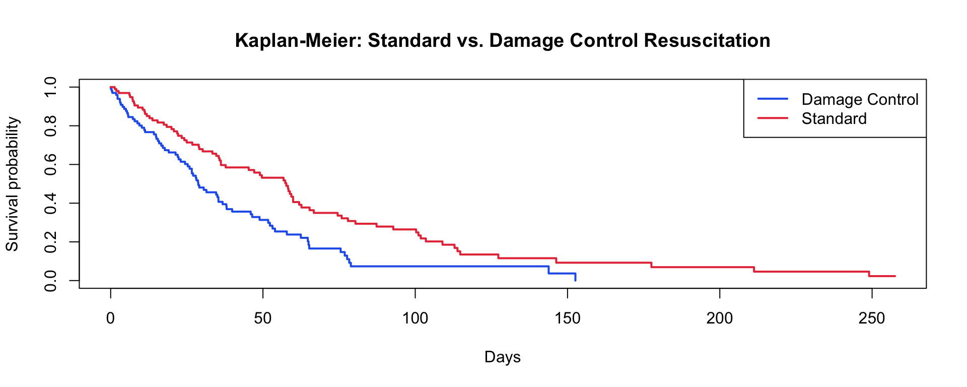
Wilcoxon Rank-Sum in Practice

group_a <- c(2,4,5,7,8,9,11,14,18,25)
group_b <- c(1,3,3,5,6,7,9,12,19,35)

wt <- wilcox.test(group_a, group_b, exact=FALSE)
cat("Wilcoxon W =", wt$statistic, "  p =", round(wt$p.value, 3))

Wilcoxon W = 57.5   p = 0.596

tibble(value=c(group_a,group_b),
       group=rep(c("A","B"),each=10)) |>
  ggplot(aes(group, value, fill=group)) +
  geom_boxplot(alpha=0.7) +
  scale_fill_manual(values=c("#2563eb","#e63946")) +
  labs(title="Wilcoxon rank-sum test",
       x="Group", y="Value") + theme_di() + theme(legend.position="none")

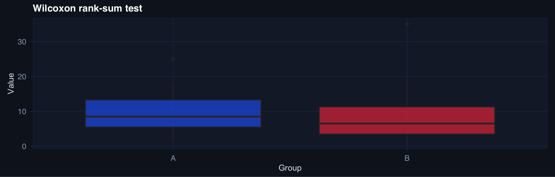
Key property: Tests whether one distribution is stochastically larger than another — doesn’t require Normality, doesn’t require equal variances.

Lecture 6 — Key Takeaways

ANOVA

• F-test = variance between / variance within
• ANOVA is a regression with group indicators
• Always correct for multiple comparisons
• Effect size: η² (eta-squared)

Survival Analysis

• Kaplan-Meier for visualization
• Log-rank test for comparison
• Cox model for adjusted hazard ratios
• Check proportional hazards assumption

Non-Parametric

• Use when Normality fails and n is small
• Rank-based → robust to outliers
• Less powerful than parametric when assumptions hold
• Spearman ρ for non-linear monotone relationships

The meta-lesson: The choice of test follows from the outcome type, sample size, and distributional assumptions — not from habit.

Coming Up: Lecture 7

Dimensionality Reduction & Clustering

Posts 15, 16, 28:

• PCA — finding the dominant directions of variation
• Clustering — grouping without labels
• Curse of Dimensionality — why high-p problems are fundamentally different

Read Before Lecture 7

• PCA Demystified
• Clustering Secrets
• Beating the Curse of Dimensionality