Model Evaluation, Ensembles & Time Series

Applied Statistics for AI & Clinical Decision-Making — Lecture 9 of 10

Jonathan D. Stallings, PhD, MS

Data InDeed | dataindeed.org

2026-01-01

Accuracy is not a metric. It’s a number that hides everything that matters.

What You’ll Learn Today

Post 29 Metrics That Matter

• ROC/AUC, precision-recall
• Calibration
• Decision curve analysis

Post 30 Ensembles

• Bagging, boosting
• Random forests
• When and why they work

Post 17 Time Series

• Autocorrelation
• ARIMA framework
• Seasonality & forecasting

Part 1

Metrics That Matter

Evaluating clinical AI like a biostatistician

Why “Accuracy” Is Misleading for Rare Events

# Trauma mortality dataset: 10% die
n <- 1000; pct_died <- 0.10
df_eval <- tibble(
  truth = c(rep(1, n*pct_died), rep(0, n*(1-pct_died))),
  pred_smart   = c(rbinom(n*pct_died, 1, 0.80), rbinom(n*(1-pct_died), 1, 0.15)),
  pred_naive   = rep(0, n)   # "never predict death" model
)

# Naive model accuracy:
cat("Naive (always 0) accuracy:", mean(df_eval$pred_naive == df_eval$truth), "\n")

Naive (always 0) accuracy: 0.9 

cat("Smart model accuracy:     ", mean(df_eval$pred_smart == df_eval$truth), "\n")

Smart model accuracy:      0.849 

A model that never predicts mortality achieves 90% accuracy on a dataset with 10% mortality. That model is useless — and dangerous. Never report accuracy alone for imbalanced clinical outcomes.

The ROC Curve and AUC

df_eval$pred_prob <- predict(
  glm(truth ~ rnorm(n) + rnorm(n), family=binomial, data=df_eval),
  type="response"
)
# Generate realistic predicted probabilities
df_eval$pred_prob <- plogis(-2 + 3*df_eval$truth + rnorm(n, 0, 1.5))

roc_obj <- roc(df_eval$truth, df_eval$pred_prob, quiet=TRUE)
plot(roc_obj, col="#2563eb", lwd=2,
     main=paste0("ROC Curve — AUC = ", round(auc(roc_obj), 3)))
abline(a=0, b=1, lty=2, col="#94a3b8")

AUC = 0.5 → random; AUC = 1.0 → perfect; AUC > 0.75 → clinically useful range.

AUC answers: “If I pick a random positive and a random negative, how often does the model rank the positive higher?” It’s threshold-independent and handles class imbalance better than accuracy. But it still doesn’t tell you if the model is well-calibrated.

Calibration: Does 30% Risk Mean 30% Mortality?

df_eval |>
  dplyr::mutate(decile = ntile(pred_prob, 10)) |>
  dplyr::group_by(decile) |>
  dplyr::summarise(mean_pred=mean(pred_prob), obs_rate=mean(truth), .groups="drop") |>
  ggplot(aes(mean_pred, obs_rate)) +
  geom_abline(linetype=2, color="#94a3b8") +
  geom_point(size=4, color="#2563eb") +
  geom_line(color="#2563eb", linewidth=1) +
  labs(title="Calibration plot — are predicted and observed rates aligned?",
       x="Mean predicted probability", y="Observed event rate") + theme_di()

A model can discriminate well (high AUC) but be poorly calibrated — predicting 20% when true risk is 50%. Always report both.

Part 2

Ensemble Methods

Many weak models → one strong model

Why Ensembles Work

Two sources of error in any single model:

• Bias — systematic wrong direction
• Variance — random fluctuation across training sets

Averaging independent models reduces variance without increasing bias.

Bagging (Bootstrap AGGregating)

• Train many models on bootstrap samples
• Average predictions
• Reduces variance
• Random Forests = bagging + random feature subsets

Boosting

• Train sequentially, each model corrects the previous
• Reduces bias
• XGBoost, LightGBM, AdaBoost
• Risk of overfitting if not regularized

Variable Importance via Lasso Coefficient Path

library(glmnet)
n <- 500
df_rf <- tibble::tibble(
  iss=rnorm(n,28,12), sbp=rnorm(n,110,20),
  gcs=rnorm(n,13,3), age=rnorm(n,35,15),
  died=rbinom(n,1,plogis(-3+0.05*iss-0.02*sbp-0.1*gcs+0.02*age))
)
X_mat <- model.matrix(died ~ iss + sbp + gcs + age, data=df_rf)[,-1]
cv_fit <- cv.glmnet(X_mat, df_rf$died, family="binomial", alpha=1, nfolds=10)

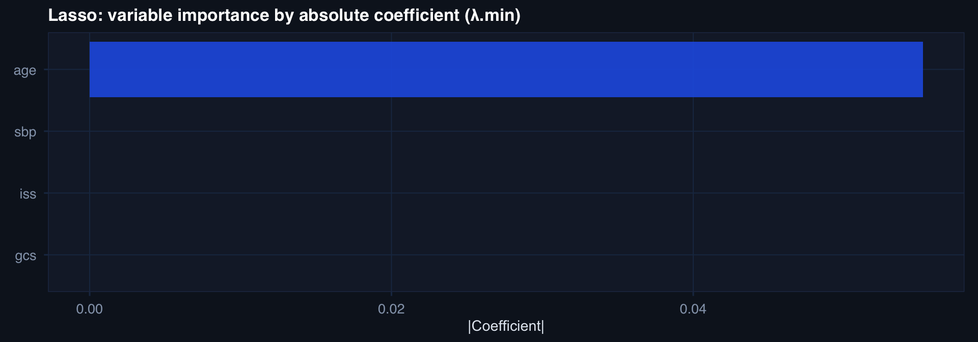
# Variable importance: absolute coefficient at lambda.min
coef_df <- as.matrix(coef(cv_fit, s="lambda.min"))[-1,,drop=FALSE]
tibble::tibble(
  Feature    = rownames(coef_df),
  Importance = abs(coef_df[,1])
) |>
  dplyr::arrange(dplyr::desc(Importance)) |>
  ggplot2::ggplot(ggplot2::aes(x=reorder(Feature,Importance), y=Importance)) +
  ggplot2::geom_col(fill="#2563eb", alpha=0.85) +
  ggplot2::coord_flip() +
  ggplot2::labs(title="Lasso: variable importance by absolute coefficient (λ.min)",
                x=NULL, y="|Coefficient|") +
  theme_di()

While random forests provide importance via mean decrease in impurity, lasso regularization offers a similarly interpretable data-driven feature ranking: features that survive at the optimal lambda are the most predictive. The absolute coefficient magnitude measures relative importance. In registry analytics with many candidate predictors, this serves the same practical purpose as random forest importance — without the need for the randomForest package.

Part 3

Time Series

When observations are ordered in time

Why Time Series Is Different

Ordinary regression assumes independence.

Time series data is autocorrelated — observations near in time are similar.

# Monthly trauma volume — seasonal + trend
time_pts <- 60
ts_data  <- tibble(
  month = 1:time_pts,
  volume = 80 + 0.3*month + 15*sin(2*pi*month/12) + rnorm(time_pts,0,8)
)
ggplot(ts_data, aes(month, volume)) +
  geom_line(linewidth=1, color="#2563eb") +
  geom_smooth(method="loess", se=FALSE, color="#e63946", linetype=2) +
  labs(title="Monthly trauma volume: trend + seasonality",
       x="Month", y="Case volume") + theme_di()

Registry monitoring: Monthly CPG compliance rates have seasonal patterns (summer injury patterns ≠ winter), baseline trends as protocols improve, and autocorrelation. Standard t-tests are invalid — time series models are required.

ARIMA: The Workhorse Time Series Model

ARIMA(p, d, q)

• AR(p): outcome depends on its own p lags
• I(d): d-order differencing for stationarity
• MA(q): outcome depends on q past errors

ts_obj <- ts(ts_data$volume, frequency=12)
fit_arima <- forecast::auto.arima(ts_obj)
summary(fit_arima)

Series: ts_obj 
ARIMA(0,0,0)(0,1,1)[12] with drift 

Coefficients:
         sma1   drift
      -0.8258  0.3161
s.e.   0.5162  0.0644

sigma^2 = 82.69:  log likelihood = -178.96
AIC=363.93   AICc=364.47   BIC=369.54

Training set error measures:
                     ME    RMSE      MAE        MPE     MAPE      MASE
Training set -0.1237474 7.96191 5.968365 -0.5790955 6.469361 0.6388639
                   ACF1
Training set -0.0949034

forecast::forecast(fit_arima, h=12) |> plot(main="12-month trauma volume forecast")

Lecture 9 — Key Takeaways

Evaluation Metrics

• Accuracy fails for imbalanced outcomes
• AUC = discrimination (rank ordering)
• Calibration = confidence accuracy
• Decision curve analysis = net benefit by threshold
• Always report both discrimination AND calibration

Ensembles

• Bagging reduces variance (Random Forests)
• Boosting reduces bias (XGBoost)
• Variable importance → data-driven feature selection
• Need cross-validation to tune — not training error

Time Series

• Autocorrelation violates independence assumption
• ARIMA(p,d,q) handles trend + autocorrelation
• Seasonality → SARIMA or seasonal decomposition
• Forecast + uncertainty interval, not point prediction

The meta-lesson: The metric you optimize shapes what your model learns to do. Choose metrics that reflect clinical consequences, not statistical convenience.

Coming Up: Lecture 10

Mathematical Foundations of Modern AI

Posts 24, 25, 26:

• Optimization — gradient descent, the engine of ML training
• Linear Algebra — vectors, matrices, SVD
• Calculus — derivatives, chain rule, backpropagation

These are the mathematical structures that sit underneath every model we’ve covered in this series.

Read Before Lecture 10

• Optimization Essentials
• Linear Algebra for Stats Pros
• Calculus Crash Course