Probability Foundations

Applied Statistics for AI & Clinical Decision-Making — Lecture 1 of 10

Jonathan D. Stallings, PhD, MS

Data InDeed | dataindeed.org

2026-01-01

Probability is not a prerequisite.

It is the language.

What You’ll Learn Today

Three posts · One lecture · ~50 minutes

Post 1 How Probability Powers AI

• What probability is
• Bayes’ theorem
• Contingency tables

Post 2 Random Variables

• Discrete vs. continuous
• Expected value & variance
• Distributions as models

Post 3 Key Distributions

• Normal, Bernoulli, Poisson
• Clinical applications
• Choosing the right one

Welcome to Lecture 1 of the Applied Statistics for AI & Clinical Decision-Making series. Today we’re covering the probabilistic foundations that every other method in this series builds on. By the end of today, you should be able to: compute basic probabilities from a contingency table, apply Bayes’ theorem, interpret a random variable and its distribution, and identify which distribution fits a given clinical or AI scenario.

Part 1

How Probability Powers AI

From spam filters to clinical triage

Why Probability? The Honest Answer

AI does not eliminate uncertainty. It formalizes decisions under uncertainty.

Every AI/ML system that outputs a “prediction” is really computing a probability:

• Email classifier: P(spam | features)
• Triage algorithm: P(deterioration | vitals, labs)
• Diagnostic model: P(injury | imaging + mechanism)

In trauma care — vitals may be incomplete, mechanism may be wrong, hemorrhage may be occult.

Probability gives us a disciplined way to reason under incomplete information.

Start by grounding this: probability is not abstract math. It’s the formal language of “I’m not sure.” Every model you’ll build in this series produces outputs that are, at their core, probabilities — even if they look like labels, risk scores, or regression coefficients.

Kolmogorov’s Three Axioms

All of probability theory rests on three rules:

Axiom 1 (Non-negativity): \(P(A) \geq 0\)

Axiom 2 (Normalization): \(P(S) = 1\)

Axiom 3 (Additivity): If A, B are mutually exclusive: \(P(A \cup B) = P(A) + P(B)\)

Why they matter for AI: A classifier that outputs incoherent probabilities (e.g., probabilities that don’t sum to 1) is mathematically invalid, not just poorly calibrated.

These three rules are not arbitrary. They are the minimum constraints needed to make probability logically consistent. Any AI model that violates them is broken, even if it looks like it’s producing output.

Joint, Marginal & Conditional Probability

The three types you’ll use constantly:

Type	Definition	Example
Joint	\(P(A \cap B)\)	P(contains “free” AND is spam)
Marginal	\(P(A) = \sum_B P(A,B)\)	P(spam) regardless of words
Conditional	\(P(A \mid B) = \frac{P(A,B)}{P(B)}\)	P(spam | contains “free”)

Trauma translation:

• Marginal = overall mortality rate in the registry
• Conditional = mortality given hemorrhagic shock AND no prehospital TXA
• Joint = probability of both shock AND ICU admission

These three types of probability appear in literally every analysis in this course. The contingency table is just a 2x2 version of the full joint probability space. Once you understand the relationship between joint, marginal, and conditional, you understand most of frequentist statistics.

Contingency Tables: Probability Engines

A 2×2 table gives you the entire joint probability space:

email_df <- tibble::tibble(
  contains_free = c("Yes","Yes","Yes","Yes","No","No","No","No","Yes","No"),
  spam          = c("Yes","Yes","No","Yes","No","No","Yes","No","Yes","No")
)

ct <- table(email_df$contains_free, email_df$spam)
prop.table(ct)        # joint probabilities

     
       No Yes
  No  0.4 0.1
  Yes 0.1 0.4

Row sums → marginal P(contains_free) Column sums → marginal P(spam) Each cell → joint P(contains_free, spam)

This is the most compact probability object there is. Once students see that a crosstab IS a joint probability matrix, everything else — Bayes, conditional distributions, independence testing — follows naturally.

Bayes’ Theorem: The Engine of Belief Updating

\[P(\theta \mid \text{data}) = \frac{P(\text{data} \mid \theta) \cdot P(\theta)}{P(\text{data})}\]

Posterior ∝ Likelihood × Prior

In clinical triage:

• Prior — baseline injury rate in this patient population
• Likelihood — how often this vital-sign pattern occurs given injury
• Posterior — updated probability of injury given what you’ve observed

Why it matters for AI:

Every Bayesian model, naive Bayes classifier, and probabilistic neural network is applying this one formula.

Bayes’ theorem is not just a formula. It is the formal description of how any rational agent — human or machine — should update their beliefs when they see new evidence. We’ll go much deeper on Bayesian methods in Lecture 4, but this is where it starts.

Quick R: Bayes’ Theorem from a Table

# Simulate: 1000 trauma patients, 15% have occult hemorrhage
# Positive FAST exam sensitivity = 0.85, specificity = 0.92

n <- 10000
p_hem    <- 0.15
sens     <- 0.85
spec     <- 0.92

# Compute positive predictive value (PPV) — Bayes in one formula
p_pos_given_hem    <- sens
p_pos_given_no_hem <- 1 - spec

p_pos <- p_pos_given_hem * p_hem + p_pos_given_no_hem * (1 - p_hem)

ppv <- (p_pos_given_hem * p_hem) / p_pos
tibble::tibble(PPV = round(ppv, 3), FDR = round(1 - ppv, 3))

# A tibble: 1 × 2
    PPV   FDR
  <dbl> <dbl>
1 0.652 0.348

This is a direct clinical application. When the base rate is 15%, even a test with good sensitivity and specificity has a false discovery rate approaching 40%. That’s the base-rate fallacy in action, and it’s one of the most common reasoning errors in clinical AI.

Part 2

Random Variables

The mathematical bridge between events and numbers

What Is a Random Variable?

A random variable maps outcomes of a random process to numbers we can compute with.

Discrete random variables Take countable values:

• Number of transfusions in 24 hrs
• Injury Severity Score (ISS)
• 30-day readmission (0 or 1)

Continuous random variables Take any value in a range:

• Systolic blood pressure
• Time to OR
• Lab values (lactate, Hgb)

The distribution of a random variable tells you how likely each value (or range of values) is.

Random variables are the building blocks of every statistical model. When we say “outcome Y” in a regression, Y is a random variable. When we say “feature X,” X is a random variable. All of statistical modeling is about understanding how random variables relate to each other.

Expected Value and Variance

Two numbers that summarize any distribution:

Expected value (mean): \(E[X] = \sum_x x \cdot P(X=x)\)

Variance: \(\text{Var}(X) = E[(X - \mu)^2]\)

Standard deviation: \(\text{SD}(X) = \sqrt{\text{Var}(X)}\)

iss_sim <- tibble::tibble(
  iss = c(9,16,25,9,4,36,16,25,9,16,25,75,9,4,16)
)
iss_sim |>
  dplyr::summarise(
    mean_iss  = mean(iss),
    sd_iss    = sd(iss),
    var_iss   = var(iss)
  )

# A tibble: 1 × 3
  mean_iss sd_iss var_iss
     <dbl>  <dbl>   <dbl>
1     19.6   17.8    315.

The expected value and variance are the two most important summaries of any distribution. In later lectures we’ll see that regression is essentially a model for the conditional expected value E[Y|X], and variance decomposition is what ANOVA is doing.

Why Variance Matters in Clinical AI

Two models with the same mean prediction can have very different clinical implications:

set.seed(123)
preds <- tibble::tibble(
  model_a = rnorm(500, mean = 0.3, sd = 0.05),
  model_b = rnorm(500, mean = 0.3, sd = 0.18)
) |>
  tidyr::pivot_longer(everything(), names_to = "model", values_to = "pred_risk")

ggplot2::ggplot(preds, ggplot2::aes(x = pred_risk, fill = model)) +
  ggplot2::geom_density(alpha = 0.5) +
  ggplot2::labs(title = "Same mean risk — very different uncertainty",
                x = "Predicted Risk", y = "Density") +
  theme_di()

Model A and Model B give the same average prediction but model B spreads predictions much wider — some patients get near-zero risk, others near-60% risk. When you’re making treatment decisions from these scores, variance is not just a statistical concept. It’s a clinical safety issue.

Part 3

Key Probability Distributions

The models behind the data

The Distribution Zoo: Which to Use When

Distribution	Data type	Classic use in trauma/AI
Bernoulli	Binary outcome (0/1)	Mortality, complication (yes/no)
Binomial	Count of successes in n trials	# of CPG-compliant cases out of 20
Poisson	Count of rare events	ED arrivals per hour, rare complications
Normal	Continuous, symmetric	Lab values, physiologic scores
Exponential	Time until event	Time to hemorrhage control
Beta	Proportions (0–1)	Prior on compliance rate
Gamma / Weibull	Skewed positive continuous	Survival time, ICU LOS

Knowing which distribution fits your outcome is not a trivial choice. Use the wrong distribution in a GLM and your predictions will be nonsensical — predicted probabilities outside 0–1, predicted counts that are negative, etc. We’ll revisit this constantly throughout the series.

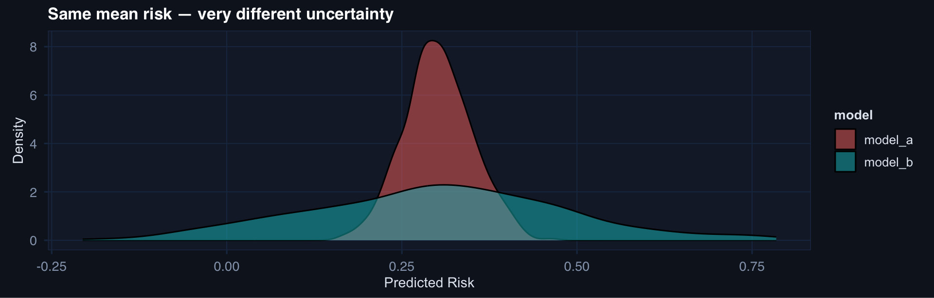
The Normal Distribution: Why It’s Everywhere

x <- seq(-4, 4, length.out = 300)

tibble::tibble(x = x, y = dnorm(x)) |>
  ggplot2::ggplot(ggplot2::aes(x, y)) +
  ggplot2::geom_line(linewidth = 1.2, color = "#2563eb") +
  ggplot2::geom_area(fill = "#2563eb", alpha = 0.12) +
  ggplot2::labs(title = "Standard Normal N(0,1)",
                x = "Standard deviations from mean", y = "Density") +
  theme_di()

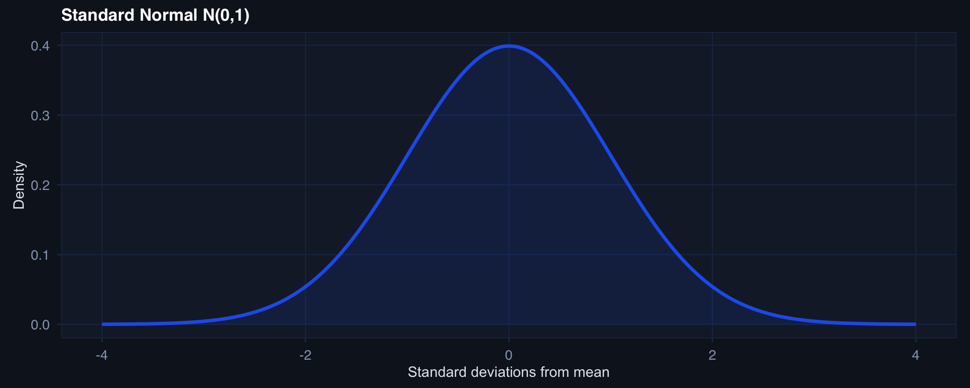
The 68-95-99.7 rule:

• 68% of data within ±1 SD
• 95% within ±2 SD
• 99.7% within ±3 SD

It’s ubiquitous because of the CLT — sums of many independent variables converge to Normal (Lecture 2).

Clinical: Systolic BP, hematocrit, temperature — all approximately Normal in stable populations.

The Normal distribution is the one that students think they understand because it shows up everywhere. But the reason it shows up everywhere is the Central Limit Theorem, which we cover in Lecture 2. For now: Normal data is symmetric, mean = median = mode, and the 2-SD interval is a 95% range.

Poisson: When Events Are Rare and Independent

lambdas <- c(1, 3, 8)
pois_df <- purrr::map_dfr(lambdas, function(l) {
  tibble::tibble(
    x = 0:20,
    prob = dpois(0:20, lambda = l),
    lambda = paste0("λ = ", l)
  )
})

ggplot2::ggplot(pois_df, ggplot2::aes(x, prob, fill = lambda)) +
  ggplot2::geom_col(position = "dodge", alpha = 0.85) +
  ggplot2::scale_fill_brewer(palette = "Blues") +
  ggplot2::labs(title = "Poisson distribution — three rates",
                x = "Count", y = "P(X = x)", fill = NULL) +
  theme_di()

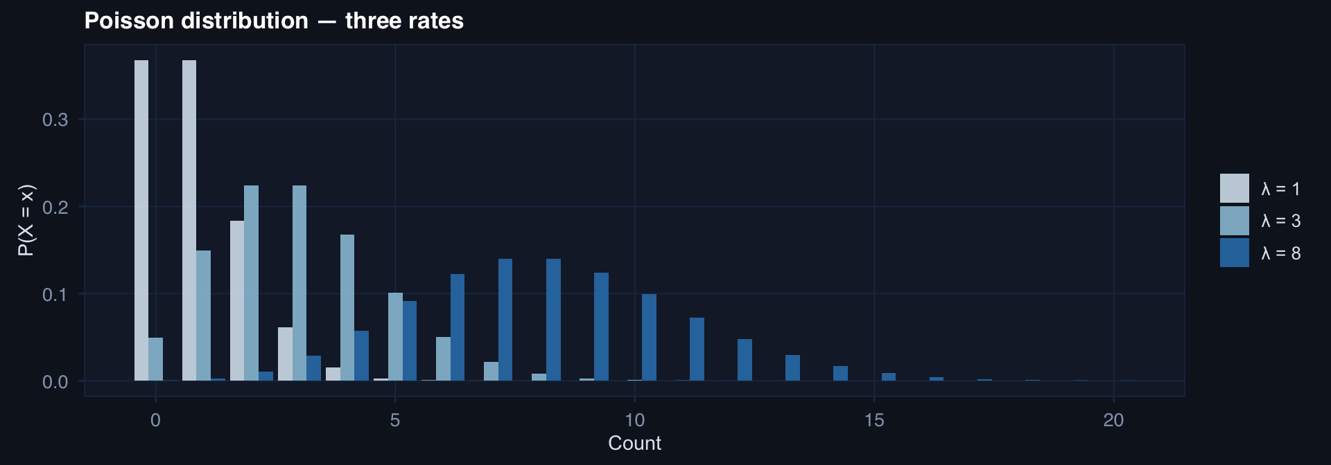
Clinical application: Rare adverse events — anastomotic leaks, intraoperative cardiac arrest, battlefield tourniquet failures. When mean ≈ variance and events are independent, Poisson is the right model.

The Poisson is the go-to distribution for count data when events are rare and independent. In CPG compliance work, if we’re counting the number of violations in a 30-day window, Poisson is almost always the starting point. Important property: E[X] = Var[X] = λ. If your data has variance much larger than the mean, you have overdispersion — which we handle with negative binomial regression.

Choosing a Distribution: The Decision Tree

Is the outcome binary (0/1)?
  → Bernoulli / Binomial

Is the outcome a count?
  → Poisson (if mean ≈ variance)
  → Negative Binomial (if overdispersed)

Is the outcome time-to-event?
  → Exponential / Weibull / Cox (Lecture 6)

Is the outcome continuous and symmetric?
  → Normal

Is the outcome continuous and right-skewed?
  → Gamma / Log-Normal

Is the outcome a proportion (0–1)?
  → Beta (as a prior) / logistic regression

This decision tree is something I want you to internalize early. By Lecture 5 (Regression), you’ll be choosing GLM families based on exactly this logic. The distribution choice is not a formality — it determines what predictions are even possible.

Lecture 1 — Key Takeaways

Probability

• Three axioms make probability coherent
• Joint, marginal, conditional are always relationships between the same numbers
• Bayes’ theorem formalizes how evidence updates belief

Random Variables

• Map events to numbers
• Discrete vs. continuous is a modeling choice
• E[X] and Var(X) summarize any distribution

Distributions

• Bernoulli/Binomial → binary and count outcomes
• Normal → symmetric continuous data
• Poisson → rare, independent events
• Exponential/Weibull → time-to-event

Clinical Application

• Every risk score is a posterior probability
• Base rates matter enormously
• Distribution choice is a scientific claim, not a formality

Coming Up: Lecture 2

The Laws That Make Statistics Work

Posts 04, 05, 06:

• CLT — why sample means become Normal, regardless of original distribution
• LLN — why bigger samples converge to truth
• Sampling — strategies, bias, sample size, design implications

These three results are why statistics can make reliable inferences from incomplete data.

Read Before Lecture 2

• The CLT Magic
• LLN in Action
• Mastering Sampling

Resources

Blog posts for this lecture:

• How Probability Powers Everyday AI
• Demystifying Random Variables
• Top Probability Distributions

Series toolkit:

• Prediction Modeling Toolkit

Data InDeed:

• dataindeed.org
• Stats series home: Applied Statistics for AI